Let's Talk Distributions Part -2
07 Sep 2020
In first part of this series we saw many distributions which arise as some variations of collection of Bernoulli trials ; binomial distribution . I mention this to make you realise that distributions are nothing but tools to make probability calculations easy and handy . The same way you could probably derive the derivative of $\sin{x}$ to be $\cos{x}$ using the first principle every time you needed it ; but its far easier to simply use the pre-derived formulae . In essence , distributions are pre-done complex probability calculations which can then be used to do many useful things; without starting from scratch .
We’ll continue our journey to find other distributions arising from variations of binomial distribution. Starting with Geometric Distribution
Geometric Distribution
Imagine that there is 10% chance that you can hit the bulls eye in a game of darts [ or make a profit on a share buy, sadly the same thing these days ]. Whats the probability that you’ll go without hitting the bulls eye for 6 consecutive throws , before eventually hitting the prize shot . Thats geometric distribution for you. Probability of $(K-1)$ consecutive failures before you see success in the $K^{th}$ trial .
\[P(x=K) = q^{k-1}p\]As we have been doing for other distributions , we’d like to calculate the mean and variance for geometric distribution also. As we have done earlier , before we jump into doing that, we’ll derive some tricky maths results and use them later.
We will start with the expression for sum of an infitite geometric series .
\[\begin{align} \sum\limits_{k=0}^\infty b^k =\frac{1}{1-b} \end{align}\]Lets differentiate on both sides $w.r.t. b$ once :
\[\begin{align} & \ \sum\limits_{k=1}^\infty kb^{k-1} =\frac{1}{(1-b)^2} \end{align}\]We’ll do this once more after multiplying both sides by $b$ once :
\[\begin{align} & \ \sum\limits_{k=1}^\infty kb^{k} =\frac{b}{(1-b)^2} \\ & \ \sum\limits_{k=1}^\infty k^2b^{k-1} =\frac{1}{(1-b)^2}+\frac{2b}{(1-b)^3} \\ & \ \sum\limits_{k=1}^\infty k^2b^{k-1} =\frac{1+b}{(1-b)^3} \end{align}\]in short, two results that we derived are :
- $\sum\limits_{k=1}^\infty k b^{k-1} =\frac{1}{(1-b)^2}$
- $\sum\limits_{k=1}^\infty k^2 b^{k-1}=\frac{(1+b)}{(1-b)^3}$
mean
\[\begin{align} \mu &= E[X] \\&= \sum\limits_{k=1}^\infty k q^{k-1}p \\&=\frac{p}{(1-q)^2}=\frac{p}{p^2}=\frac{1}{p} \end{align}\]This simply implies that if you have 15% chance to hit the bulls eye, on an average ; it will take you $\frac{1}{.15} \sim 7$ attempts to get that shot .
Variance
\[\begin{align} E[X^2]&=\sum\limits_{k=1}^\infty k^2 q^{k-1}p \\&= \frac{p(1+q)}{(1-q)^3}=\frac{1+q}{p^2} \end{align}\] \[\begin{align} Var(X) &= E[X^2]-(E[X])^2 \\&=\frac{1+q}{p^2}-\frac{1}{p^2}=\frac{q}{p^2} \end{align}\]and the variance in this number , number of attempts that it takes people to get first success is going to be $\frac{0.85}{0.15^2} \sim 37$ , which is a huge number especially in comparison to the average number of trials it’s going to take. Insight that you should derive from here is that , for a low success task, don’t be deceived by a small average , be vary of the variance .
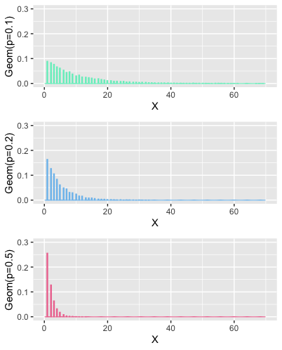
what does it look like
The only parameter this distribution has, is $p$ .

Notice that for low success scenarios , probability of early success is low , and the chance of getting success later, extends much farther in comparison to high success rate scenarios. Variance is also low for high success scenarios .
HyperGeometric Distribution
In the scenarios discussed so far, we have not considered the case of finite population . Consider this question, if a city of 10000 residents has 200 doctors . Whats the probability that out of 100 randomly selected citizens , 10 are doctors .
A generic formula to answer this question will consider, Population size = N, number of successes present in the population = M, Size of the sample being taken = n . then
\[P(X=x)=\frac{\binom{M}{x}*\binom{N-M}{n-x}}{\binom{N}{n}}\]This is our hypergeometric distribution. note that there is a limit on value of $x$ and $n$ here , since the population is finite . $n\in [1,N]$ and $x \in [0,n]$ .
time for deriving maths results for using later
\[\begin{align} r*\binom{n}{r}&=\frac{r * n!}{r!* (n-r)!} \\ &=\frac {n*(n-1)!}{(r-1)!(n-1-(r-1))!} \\&=n*\binom{n-1}{r-1} \end{align}\]mean
\[\begin{align} E[X]&=\sum\limits_{x=1}^{n}\frac{x*\binom{M}{x}*\binom{N-M}{n-x}}{\binom{N}{n}} \\ &=\sum\limits_{x=1}^{n}\frac{M*\binom{M-1}{x-1}*\binom{N-M}{n-x}}{\binom{N}{n}} \\&=\sum\limits_{x=1}^{n}\frac{M*\binom{M-1}{x-1}*\binom{N-1-(M-1)}{n-1-(x-1)}}{\binom{N}{n}} \\ &=\frac{M}{\binom{N}{n}}*\binom{N-1}{n-1}\sum\limits_{x=1}^{n}\frac{\binom{M-1}{x-1}*\binom{N-1-(M-1)}{n-1-(x-1)}}{\binom{N-1}{n-1}} \end{align}\]The expression written inside the summation here is another hypergeometric distribution with parameters $N-1$ , $M-1$ and $n-1$ . This pmf summed over all values of $x$ will simply be 1.
\[\begin{align} E[X]&=\frac{M}{\binom{N}{n}}*\binom{N-1}{n-1}\sum\limits_{x=1}^{n}\frac{\binom{M-1}{x-1}*\binom{N-1-(M-1)}{n-1-(x-1)}}{\binom{N-1}{n-1}} \\&=\frac{M}{\binom{N}{n}}*\binom{N-1}{n-1} \\&=\frac{M*n!*(N-n)!}{N!}*\frac{(N-1)!}{(n-1)!(N-n)!} \\&=\frac{M*n}{N} \end{align}\]Now if you think about it , $\frac{M}{N}$ is the probability of success and the result that you see above is simply $np$ , same as what we got for binomial distribution .
Variance
\[\begin{align} E[X^2]&=\sum\limits_{x=1}^{n}\frac{x^2*\binom{M}{x}*\binom{N-M}{n-x}}{\binom{N}{n}} \\ &= \sum\limits_{x=1}^{n}\frac{x*M*\binom{M-1}{x-1}*\binom{N-M}{n-x}}{\binom{N}{n}} \\ &= \sum\limits_{x=1}^{n}\frac{(x-1+1)*M*\binom{M-1}{x-1}*\binom{N-M}{n-x}}{\binom{N}{n}} \\&= \sum\limits_{x=1}^{n}\frac{(x-1)*M*\binom{M-1}{x-1}*\binom{N-M}{n-x}}{\binom{N}{n}}+\sum\limits_{x=1}^{n}\frac{M*\binom{M-1}{x-1}*\binom{N-M}{n-x}}{\binom{N}{n}} \\&= \sum\limits_{x=1}^{n}\frac{M*(M-1)\binom{M-2}{x-2}*\binom{N-M}{n-x}}{\binom{N}{n}} +\frac{M*\binom{N-1}{n-1}}{\binom{N}{n}}\sum\limits_{x=1}^{n}\frac{\binom{M-1}{x-1}*\binom{N-M}{n-x}}{\binom{N-1}{n-1}} \\&= \frac{M*(M-1)*\binom{N-2}{n-2}}{\binom{N}{n}}\sum\limits_{x=1}^{n}\frac{\binom{M-2}{x-2}*\binom{N-2-(M-2)}{n-2-(x-2)}}{\binom{N-2}{n-2}} +\frac{M*\binom{N-1}{n-1}}{\binom{N}{n}}\sum\limits_{x=1}^{n}\frac{\binom{M-1}{x-1}*\binom{N-1-(M-1)}{n-1-(x-1)}}{\binom{N-1}{n-1}} \end{align}\]The first summation is pmf of a hypergeometric distribution with parameters $N-2$,$M-2$,$n-2$ ;the second term is the same but with parameters $N-1$,$M-1$,$n-1$ . Both of them will sum up to 1 .
\[\begin{align} E[X^2]&= \frac{M*(M-1)*\binom{N-2}{n-2}}{\binom{N}{n}}\sum\limits_{x=1}^{n}\frac{\binom{M-2}{x-2}*\binom{N-2-(M-2)}{n-2-(x-2)}}{\binom{N-2}{n-2}} +\frac{M*\binom{N-1}{n-1}}{\binom{N}{n}}\sum\limits_{x=1}^{n}\frac{\binom{M-1}{x-1}*\binom{N-1-(M-1)}{n-1-(x-1)}}{\binom{N-1}{n-1}} \\&=\frac{M*(M-1)*\binom{N-2}{n-2}}{\binom{N}{n}} +\frac{M*\binom{N-1}{n-1}}{\binom{N}{n}} \\&=\frac{M*(M-1)*(N-2)!n!(N-n)!}{(n-2)!(N-n)!N!}+\frac{M*(N-1)!n!(N-n)!}{N!(n-1)!(N-n)!} \\&=\frac{M*(M-1)*n*(n-1)}{N*(N-1)}+\frac{M*n}{N} \\&=\frac{M*n}{N}\Big[\frac{(M-1)*(n-1)}{N-1}+1\Big] \end{align}\]Now that we have managed to get this , lets go to the variance
\[\begin{align} Var(X)&=E[X^2]-(E[X])^2 \\&=\frac{M*n}{N}\Big[\frac{(M-1)*(n-1)}{N-1}+1\Big] -\frac{M^2*n^2}{N^2} \\&=\frac{M*n}{N}\Big[\frac{(M-1)*(n-1)}{N-1}+1-\frac{M*n}{N}\Big] \\&=\frac{M*n}{N}\Big[\frac{M*n*N-M*N-n*N+N+N^2-N-M*n*N+M*n}{N*(N-1)}\Big] \\&=\frac{M*n}{N}\Big[\frac{-M*N-n*N+N^2+M*n}{N*(N-1)}\Big] \\&=\frac{M*n}{N}\Big[\frac{N*(N-n)-M*(N-n)}{N*(N-1)}\Big] \\&=\frac{M*n}{N}\Big[\frac{(N-M)*(N-n)}{N*(N-1)}\Big] \\&=n*\frac{M}{N}*\Big(1-\frac{M}{N}\Big)\frac{(N-n)}{(N-1)} \end{align}\]This again is close to $npq$ ; which was the variance of binomial distribution . [considering $\frac{M}{N}=p$], however it comes with correction factor $\frac{N-n}{N-1}$; also known as finite population correction factor for binomial distribution .
Another way to differentiate between binomial distribution and hypergeometric distribution is to look at hypergeometric distribution as the result of sampling without replacement and binomial distribution to be sampling with replacement [letting go of the constraints on population size].
I am skipping the what does it look like section here as the visuals are mostly going to be like binomial distribution.
Negative Binomial Distribution
Recall that, binomial variable was defined as number of successes you might get to see in fixed number of trials . What if we now want to consider a scenario where number of successes are fixed and we would like to know, how many trials it will take to reach there .
\[P(X=x)=\binom{x-1}{r-1}*p^r*q^{(x-r)}\]There is another more common expression for this distribution; which makes further calculations rather convenient and thats the expression where the distribution derives its name from .Instead of looking at number of trials required [say $x$] to reach $r$ successes, we’ll use number of failures [say $y$] before $r^{th}$ success . This relationship holds between this $x$ and $y$ .
\[y=x-r\]and pmf for this variable is given by
\[P(Y=y)=\binom{y+r-1}{y}*p^r*q^{y}\]The binomial coefficient that you see here appears in negative binomial expressions , that is where the name comes from. Next we are going to derive some maths to make our job easy later while calculating mean and variance of these distributions .
\[\begin{align} \binom{y+r-1}{y}&=\frac{(y+r-1)(y+r-2)(y+r-3)\cdots r(r-1)(r-2)\cdots3*2*1}{y!(r-1)!} \\&=\frac{(y+r-1)(y+r-2)(y+r-3)\cdots r}{y!} \\&=(-1)^y\frac{(-r)(-r-1)\cdots(-r-(y-1))}{y!} \\&=(-1)^y*\binom{-r}{y} \end{align}\]Next bit we will start with Taylor’s expansion of a function :
\[f(x)=\sum_{k=0}^\infty f^{(k)}(a)\frac{(x-a)^k}{k!}\]Where $ f^{(k)} $ is $ k^{th} $ derivative of $f$ and $x\to a$. Now consider $a=0$ . That makes the above expression a maclaurin series [ putting the name here , so that you can go explore more if you are interested] . Since we are considering $a$ to be $0$ here , this will work for $x \to 0$ , or $\lvert x \rvert <1 $ .
\[f(x)=\sum_{k=0}^\infty f^{(k)}(0)\frac{x^k}{k!}\]Lets consider a special function to use this for :
\[\begin{align} & 1. \ f(x)=(1-x)^{-r} \\& 2. \ f^{(k)}(x) =(-1)^k (-r)*(-r-1)*(-r-2)\cdots*(-r-(k-1))(1-x)^{(-r-k)} \\& 3. \ f^{(k)}(0) =(-1)^k (-r)*(-r-1)*(-r-2)\cdots*(-r-(k-1)) \end{align}\]Using the maclaurin series given above we can write :
\[\begin{align} (1-x)^{-r}&=\sum_{k=0}^\infty (-1)^k \frac{(-r)*(-r-1)*(-r-2)\cdots*(-r-(k-1))}{k!}*x^k \\ &=\sum\limits_{k=0}^\infty (-1)^k *\binom{-r}{k}*x^k \end{align}\]Lets differentiate this $w.r.t. \ x$ once on both sides
\[\begin{align} & \ r(1-x)^{-r-1}=\sum\limits_{k=0}^\infty (-1)^k *k*\binom{-r}{k}*x^{k-1} \\ & \ rx(1-x)^{-r-1}=\sum\limits_{k=0}^\infty (-1)^k *k*\binom{-r}{k}*x^{k} \end{align}\]Once more :
\[\begin{align} & \ r(1-x)^{-r-1}+rx(r+1)(1-x)^{-r-2}=\sum\limits_{k=0}^\infty (-1)^k *k^2*\binom{-r}{k}*x^{k-1} \\& \ rx(1-x)^{-r-1}+rx^2(r+1)(1-x)^{-r-2}=\sum\limits_{k=0}^\infty (-1)^k *k^2*\binom{-r}{k}*x^{k} \\& \ rx(1-x+rx+x)(1-x)^{-r-2}=\sum\limits_{k=0}^\infty (-1)^k *k^2*\binom{-r}{k}*x^{k} \\& \ rx(rx+1)(1-x)^{-r-2}=\sum\limits_{k=0}^\infty (-1)^k *k^2*\binom{-r}{k}*x^{k} \end{align}\]Summarising results that we will be using :
\[\begin{align} & 1. \ \binom{y+r-1}{y} = (-1)^y*\binom{-r}{y} \\ & 2. \ (1-x)^{-r} = \sum\limits_{k=0}^\infty (-1)^k *\binom{-r}{k}*x^k \\ & 3. \ \sum\limits_{k=0}^\infty (-1)^k *k*\binom{-r}{k}*x^{k}=rx(1-x)^{-r-1} \\ & 4. \ \sum\limits_{k=0}^\infty (-1)^k *k^2*\binom{-r}{k}*x^{k}=(rx+1)rx(1-x)^{-r-2} \end{align}\]Mean
\[\begin{align} E[Y]&=\sum\limits_{y=0}^\infty y*\binom{y+r-1}{y}*p^r*q^{y} \\&=\sum\limits_{y=0}^\infty (-1)^{y}*y*\binom{-r}{y}*p^r*q^{y} \\&=p^r\sum\limits_{y=0}^\infty (-1)^{y}*y*\binom{-r}{y}*q^{y} \\&=p^r*r*q(1-q)^{-r-1}=p^r*r*q*p^{-r-1}=\frac{rq}{p} \end{align}\]If you need to hit the bullseye at-least 3 times in the same night to appear on the hall of fame board of the bar , how many times on an average you need to try throwing darts; given that the probability of you hitting the bulls eye is $\frac{1}{10}$ . Using the result above , the answer comes to be $\frac{3*\frac{9}{10}}{\frac{1}{10}} = 42$ , that is average number of failures , before the 3rd success, meaning $42+3=45$ trials , before you make it to the hall of fame. Woah, you better get really good at darts , or just be patients , or may be not so ambitious otherwise . Life has other things to offer, you just need to look beyond the ….Bulls eye.
Variance
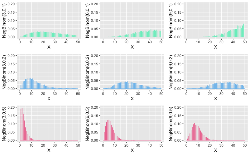
\[\begin{align} E[Y^2]&=\sum\limits_{y=0}^\infty y^2*\binom{y+r-1}{y}*p^r*q^{y} \\&=p^r\sum\limits_{y=0}^\infty y^2*\binom{y+r-1}{y}*q^{y} \\&=p^r\sum\limits_{y=0}^\infty (-1)^y*y^2*\binom{-r}{y}*q^{y} \\&=p^r(rq+1)*r*q*p^{-r-2} \\&=(rq+1)\frac{rq}{p^2} \end{align}\] \[\begin{align} Var[Y]&=E[Y^2]-(E[Y])^2 \\&=(rq+1)\frac{rq}{p^2}-\frac{r^2q^2}{p^2} \\&=\frac{rq}{p^2}(rq+1-rq)=\frac{rq}{p^2} \end{align}\]what does it look like

See, how low success rate scenarios end up being very flat , positively skewed and fat tailed , for low number of success. And as number of successes start to go up, distribution for high success scenarios also start to shift to right, but much slower.
Concluding this post
So far our discussions on this series have been mostly on discrete distributions [Exponential distribution , briefly popped up towards the end of the last post]. In the next post, we’ll be going to unravel mysteries of continuous distributions. Where they come from, how can we understand them; both as limiting cases of discrete distributions, as well as relate them to real life continuous data.
If you haven’t read the first part , here it is
