
Let's Talk Distributions Part -1
07 Jul 2020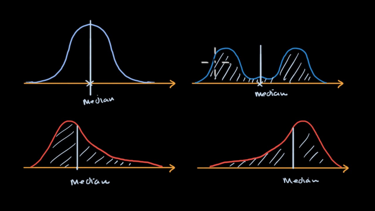
All the distributions that we will discuss, can be categorised into two broad groups : Discrete and Continuous .
- Discrete distributions pertain to data which contains discrete outcomes [Integers] as their values. E.g. Number of people on the train , Count of bees in an honeycomb . [Imagine the horror of seeing three and quarter of a person getting off the train!]
- Continuous distributions on the other hand have values which can take values in decimals . E.g. Weight of students in a class, Length of trees in a forest [Number of people in a zombie movie?]
We’ll start our discussion with a very simple and intuitive distribution known as uniform distribution . In that discussion we will also learn about defining and calculating mean and variance as Expectation.
Uniform Distribution [Discrete]
Uniform distribution is where each value in the distribution has equal probability of occurrence . If we had to come up with a general expression for probability of occurrence of each value in the uniform distribution, we can write .
\[P(X=x) = \frac{1}{n}\]Where n is the number of values in the range of the distribution. A classic example which produces uniform distribution is throwing a fair dice. 🎲
Each throw might result in any of the $ {1,2,3,4,5,6}$ on the top face with equal probability . So in this case
\[P(X=x)=\frac{1}{6} \ \ \forall \ x \in \{1,2,3,4,5,6\}\]Expectation
Consider a gambling party where the host has gone bonkers and is asking guests to throw a dice and collect as much money as the number which shows on the face of the dice. However if you get 1 , you have to give $ 10 to the host.On an Average how much money the host is going to make [or lose] on each player.
We can start by assuming there are 72 [ the number doesn’t really matter ] people in the party . Since the dice is fair; we can assume that each of ${1,2,3,4,5,6}$ will be obtained by 12 guests.
- So the money lost by host $ {=12X6 + 12X 5 + 12X4 +12X3 +12X2 = $ 240} $
- money gained by host $=12X10 = $120$
- Overall money lost by host $= 240 - 120 = $120$
- Money lost per player $\frac{$120}{72}=$1.67$
A simpler way of doing this will be to multiply probability of each outcome with the outcome and sum them.
Average gain
\(=-6*\frac{1}{6}-5*\frac{1}{6}-4*\frac{1}{6}-3**\frac{1}{6}-2*\frac{1}{6}+10*\frac{1}{6}=\$1.67\)$
This is also known as expected value of a distribution [or mean]. A formal expression for the same will be
\[\mu = E[X] = \sum xP(X=x)\]Let’s calculate mean of uniform distribution like this . Say distribution takes integer values in the interval $[a,b]$ with $n$ values in it.
[$b = a + (n-1)$], Since $b$ is the $n^{th}$ element .
\[\begin{align} \mu & = E[X] \\ & =[a+(a+1)+(a+2).....+b]*\frac{1}{n} \\ & = [n*a + (1+2+3....n-1)]*\frac{1}{n} \\ & = [n*a + (n-1)*\frac{n}{2} ]*\frac{1}{n} \\ & =\frac{2a+n-1}{2} \\ & =\frac{a+a+n-1}{2} \\ & =\frac{a+b}{2} \end{align}\]Before we proceed further I will mention here few algebraic properties of expectation which are easy to derive; so I am going to put them here without extensive proof.
- $E[g(X)] = \sum g(x)P(X=x)$
- $E[const]=const$
- $E(aX+b) = aE(X)+b$
Variance of a distribution is defined as expectation of $(X-\mu)^2$ . [remember variance was mean of squared deviations from the mean]
\[\begin{align} Var(X)&=E[(X-\mu)^2] \\ &= E[X^2 + \mu^2 - 2\mu X] \\ &= E[X^2]+\mu^2-2\mu E[X] \\&= E[X^2]-\mu^2 \\&=E[X^2]-(E[X])^2 \end{align}\]Lets calculate variance of uniform distribution with this
\[\begin{align} E(X^2)&=[a^2+(a+1)^2+.......(a+n-1)^2]*\frac{1}{n} \\ & = [n*a^2 + (1+2^2+3^2+......(n-1)^2) - 2*a(1+2+3....n-1)]*\frac{1}{n} \\ & = [n*a^2 + \frac{(n-1)n(2n-1)}{6}-2*a*\frac{(n-1)(n)}{2}]*\frac{1}{n} \\ & = a^2 + \frac{(b-a)(b-a+1)(2b-2a+1)}{6}-a(b-a)(b-a+1) \\ &\;\;\vdots \\ Var(X) & = E(X^2)-[E(X)]^2 \\ & = \frac{(b-a)^2}{12} \end{align}\]I have skipped some algebraic gymnastic there. Do it yourself if it rubbed your marbles the wrong way.
For continuous distributions ; if the pdf is given as $f(x)$ then
- $E[X]=\int xf(x)dx$
Key Takeaways
About expectations :
- $E[X]=\sum xP(X=x) = \int xf(x)dx$
- $Var(X)=E[X^2]-(E[X])^2$
About discrete uniform distribution :
- $P(X=x)=\frac{1}{n} \forall x \in {a,a+1,…b} \ with \ n \ elements$
- $\mu = E(X) = \frac{(a+b)}{2}$
- $Var(X) = \frac{(b-a)^2}{12}$
What does it look like
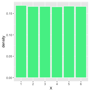
Bernoulli’s Distribution [Discrete]
We get a call on our phone , we receive it or we don’t . We are driving on the road , we reach home safely or we die [ well that went from 0 to dead pretty fast] . Life is full of transactions which have two outcomes . 0/1 , failure/success, accept/decline and so on.
And each of these outcomes have some associated probability . Like there is 90% chance of an advice being solid gold if given by an old dude while peeling an apple with a pocket knife and eating pieces right off the blade . Oddly specific but relatable.
Formally we write :
\[P(X=x) = \begin{cases} p & \text{ if x =1} \\ q & \text{ if x =0, where q =1-p} \end{cases}\]Mean
\[\begin{align} \mu &= E[X] \\ &= 1 * p + 0*q \\ & =p \end{align}\]Variance
\[\begin{align} E[X^2] & = 1^2 * p + 0^2*q \\&=p \\Var(X) &= E[X^2]-[E[X]]^2 \\&=p-p^2=p*(1-p) \\&=pq \end{align}\]What does it look like
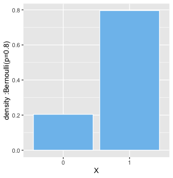
Life is nothing but a sequence of countless Bernoulli Trials .
Binomial Distribution [Discrete]
During the pandemic lockdown, you have learnt to make absolutely killer cocktails. Probability of a person getting shitfaced drunk on the cocktail is $p$ . Let’s say $n$ people attended your party once the lockdown opens , what are the chances that $x$ of them will have no memory of what happened that night ?
$x$ is just number of guests . It can be made up of any $x$ guests out of $n$ . We can chose $x$ guests out of $n$ in ${}^{n}C_{x}$ ways.
\[\begin{align} {}^{n}C_{x} &= \frac{!n}{!x!(n-x)} \\ \\ \text{given }!n &= n*n(n-1)\cdots2*1 \end{align}\]formally we can write [considering $q=1-p$]
\[P(X=x) = {}^{n}C_{x} * p^x *q^{n-x}\]Before we get down to calculating mean and variance , let’s get done with some mean looking maths involving binomial coefficients .
We know that $(a+b)^n$ can be expanded using following expression involving binomial coefficients .
\[(a+b)^n = \sum\limits_{r=0}^{n}{}^{n}C_{r}a^r b^{n-r}\]Now to the mean maths; we are going to derive some results which will come in handy later.
\[\begin{align} \sum\limits_{r=0}^{n} r *{}^{n}C_{r} * a^r *b^{n-r} &= a* \sum\limits_{r=0}^{n} r *{}^{n}C_{r} * a^{r-1} *b^{n-r} \\&= a*\frac{d}{da}[\sum\limits_{r=0}^{n} {}^{n}C_{r} * a^r *b^{n-r}] \\&=a*\frac{d}{da}[(a+b)^n] \\&=na(a+b)^{n-1} \\ \sum\limits_{r=0}^{n} r^2 *{}^{n}C_{r} * a^r *b^{n-r} &= \sum\limits_{r=0}^{n} r(r-1) *{}^{n}C_{r} * a^r *b^{n-r}+\sum\limits_{r=0}^{n} r *{}^{n}C_{r} * a^r *b^{n-r} \\&=a^2\sum\limits_{r=0}^{n} r(r-1) *{}^{n}C_{r} * a^{r-2} *b^{n-r}+na(a+b)^{n-1} \\&=a^2*\frac{d}{da}[\sum\limits_{r=0}^{n} r *{}^{n}C_{r} * a^{r-1} *b^{n-r}]+na(a+b)^{n-1} \\&=a^2*\frac{d}{da}[\frac{d}{da}[\sum\limits_{r=0}^{n} {}^{n}C_{r} * a^{r} *b^{n-r}]]+na(a+b)^{n-1} \\&=a^2*\frac{d}{da}[\frac{d}{da}[(a+b)^n]]+na(a+b)^{n-1} \\&=n(n-1)a^2(a+b)^{n-2}+na(a+b)^{n-1} \end{align}\]Mean
\[\begin{align} \mu &= E[X] \\ &= \sum\limits_{x=0}^{n} x *{}^{n}C_{x} * p^x *q^{n-x} \\&=np(p+q)^{n-1} \\&=np \ \ \ [\text{since $p+q=1$}] \end{align}\]Variance
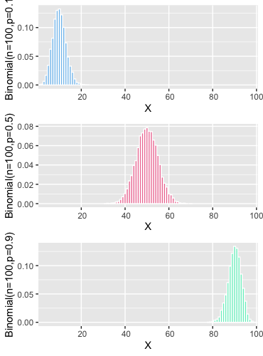
\[\begin{align} E[X^2] &=\sum\limits_{r=0}^{n} x^2 *{}^{n}C_{x} * p^x *q^{n-x} \\&=n(n-1)p^2(p+q)^{n-2}+np(p+q)^{n-1} \\&=n(n-1)p^2+np \\Var(X) &=E[X^2]-[E[X]]^2 \\&=n(n-1)p^2+np-n^2p^2 \\&=np(1-p) \\&=npq \end{align}\]What does it look like
CDF [cumulative density function]
Many at times , probability of an instance is not very useful. And it’s better to have a look at probability of an interval instead . This can be calculated as difference between cumulative probabilities which are defined as follows [given that X takes values in the interval $[a,b]$]
- for discrete distribution $CDF = P(X\le x) = \sum\limits_{x=a}^{x}P(X=x)$
- for continuous distributions = $\int\limits_{a}^{x}f(x)dx$
An Example
for a large clinical trial where there were 1000 patients and probability of success was 20% . answer following questions [I have added R codes, wherever needed]
- whats the expected number of cured patients = np = 1000*0.2=200
- whats the expected standard deviation across multiple such clinical trials $= \sqrt{npq}=\sqrt{1000X0.2X0.8} =12.6$
# whats the probability that 200 of the patients will be cured
dbinom(200,1000,0.2)

# whats the probability that upto 200 patients will be cured [use functions for cdf]
pbinom(200,1000,0.2)

# whats the probability that number of patients cured
# will be between 190 and 210 [use function for cdf]
pbinom(210,1000,0.2)-pbinom(190,1000,0.2)
I did not explicitly mention, but I hope you realised that Binomial Distribution is collection of Bernoulli trials . Where each individual outcome is from Bernoulli distribution. Binomial Distribution’s outcome is nothing but sum of the outcomes of those Bernoulli trials.
Poisson Distribution [Discrete]
You hear the unsavoury news that someone found an iron nail in their sausage and suddenly everyone in the group starts recounting similar experiences; and makes you feel as if this has become a very common phenomenon and world has gone to dogs and its a mistake to become a parent in these times and blah blah blah .
But if you take a step back and for a moment consider that; millions of sausages are consumed everyday and you rarely get to hear about someone really finding a nail in theirs. Mostly because, not finding a nail in your sausage is not NEWS, but finding a nail means; hell has finally frozen over. Same as a thousands of cars mundanely passing a town centre do not become talk of the town, but a single accident does.
I did not take this crazy sounding; sudden tangent in our discussion to play down the risk of nails or accident. The strange take aways that i want you to have from following news bite : ` there were 5 accidents last month in this traffic junction` are :
- We don’t know whats the probability of an individual vehicle passing the junction getting into an accident , but we do know that its pretty small despite the hullabaloo about the accidents
- We also know that thousands of vehicle must have passed through the junction which eventually resulted in these 5 accidents. But we don’t know the exact value of $n$ either.
So this month of 5 accidents was essentially a huge collection of Bernoulli trials with a very small probability of success. Basically this value 5 is coming from a Binomial distribution with very large $n$ and very small $p$
We’ll call this 5 accidents/month to be rate of events and denote it with symbol $\lambda$
\[\begin{align} \lambda&=np \\ p &= \frac{\lambda}{n} \end{align}\]Now with this information, someone asks you, can you tell me whats the probability that we’ll see $x$ accidents next month [given that flow of vehicles through the junction remains similar and other traffic conditions also remain unchanged]. Let’s try to answer that question in absence of information of both $n$ and $p$ . All that we have, is the rate $\lambda$ and hunch that $n$ is large and $p$ is small.
But it still is a binomial distribution . [well for now at-least , but we are going in for the kill boys!]
\[\begin{align} \lim\limits_{n\to\infty} P(X=x) &= \lim\limits_{n\to\infty}{}^{n}C_{x} * p^x *q^{n-x} \\&=\lim\limits_{n\to\infty}\frac{!n}{!x!(n-x)} * \Big(\frac{\lambda}{n}\Big)^{x}* \Big(1-\frac{\lambda}{n}\Big)^{n-x} \\&=\frac{\lambda^x}{!x}\lim\limits_{n\to\infty}\frac{!n}{!(n-x)}*\frac{1}{n^x} * \Big(1-\frac{\lambda}{n}\Big)^{n}*\Big(1-\frac{\lambda}{n}\Big)^{-x} \end{align}\]Ah i guess we are stuck now. We’ll have to kill this beast in parts and then come back and put together it all.
\[\begin{align} \lim\limits_{n\to\infty}\frac{!n}{!(n-x)}*\frac{1}{n^x} &= \frac{n*(n-1)*\cdots*(n-x+1)*(n-x)*\cdots2*1}{[(n-x)*\cdots*2*1]*[n*n*\cdots*n]} \\&=1*\Big(1-\frac{1}{n}\Big)*\Big(1-\frac{2}{n}\Big)*\cdots*\Big(1-\frac{x-1}{n}\Big) \\&=1 \end{align}\]thats one down
\[\begin{align} e&=\lim\limits_{n\to\infty}\Big(1+\frac{1}{n}\Big)^n \\\lim\limits_{n\to\infty}\Big(1-\frac{\lambda}{n}\Big)^n&=\lim\limits_{n\to\infty}\Big[\Big(1+\frac{1}{-(n/\lambda)}\Big)^{-n/\lambda}\Big]^{-\lambda} \\&=e^{-\lambda} \end{align}\]the remaining guy is just a formality now
\[\lim\limits_{n\to\infty}\Big(1-\frac{\lambda}{n}\Big)^{-x}=1^{-x}=1\]Putting all this together we get
\[\lim\limits_{n\to\infty} P(X=x) =\frac{\lambda^x*e^{-\lambda}}{!x}\]Thats the density function for Poisson Distribution
Mean
\[\begin{align} \mu &= E[X] \\&=\sum\limits_{x=1}^{\infty}\frac{x*\lambda^x*e^{-\lambda}}{!x} \\&=\lambda*e^{-\lambda}\sum\limits_{x=1}^{\infty}\frac{\lambda^{x-1}}{!(x-1)} \\&=\lambda*e^{-\lambda}\Big[1+\frac{\lambda}{!1}+\frac{\lambda^2}{!2}+\frac{\lambda^3}{!3}\cdots\Big] \\&=\lambda*e^{-\lambda}e^{\lambda} \\&=\lambda \end{align}\]Variance
\[\begin{align} E[X^2]&=\sum\limits_{x=1}^{\infty}\frac{x^2*\lambda^x*e^{-\lambda}}{!x} \\&=\sum\limits_{x=1}^{\infty}\frac{x*(x-1)*\lambda^x*e^{-\lambda}}{!x}+\sum\limits_{x=1}^{\infty}\frac{x*\lambda^x*e^{-\lambda}}{!x} \\&=\lambda^2*e^{-\lambda}\sum\limits_{x=2}^{\infty}\frac{\lambda^{x-2}}{!(x-2)}+\lambda \\&=\lambda^2+\lambda \\Var(X)&=E[X^2]-[E[X]]^2 \\&=\lambda^2+\lambda-\lambda^2 \\&=\lambda \end{align}\]What does it look like
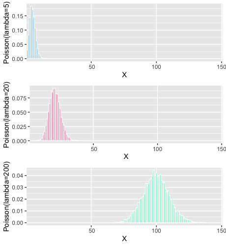
Notice, since variance is $\lambda$ , for higher values of $\lambda$ ; the distribution is becoming more spread out.
An Example
A McDonald’s on an highway receives 20 orders per hour . If that exceeds 25, they’d need to hire another person. Whats the probability that they’d need to do so.
- the cdf with x=25 here will give us probability of number of orders being upto 25
- we need probability of $x\ge25$
1-ppois(25,20)
Exponential Distribution [Continuous]
You know; the fear [ father of all the questions, doubts and drugs ] is not always about how many. It’s about, more often than not , when the first/next would happen. As in the first heart attack , the next kiss, [an odd couple indeed], the first covid positive patient and of-course; for the dinosaurs, the next big meteor.
Continuing with the example that we took above; what if the question that we want to answer is : whats the probability that they will receive their next order within 30 mins
Of course the answer isn’t that straight forward to come by.
We know that, events are happening at the rate $\lambda$ per unit time. So, in $t$ time units , events will happen at the rate $\lambda t$
Using Poisson distribution, probability of x events happening in next $t$ time units
\[P(X=x)=\frac{e^{-\lambda t}*(\lambda t)^x}{!x}\]Whats the probability that no event will happen in next t time units?
\[P(X=0)=e^{-\lambda t}\]Whats the probability that at-least 1 event will happen in t time units ?
\[1-P(X=0) = 1-e^{-\lambda t}\]Hey, but thats cumulative probability or in other words
\[P(T\le t)=1-e^{-\lambda t}\]and if the distribution of $t$ was defined by function $f(t)$ , we could write
\[\begin{align} \int\limits_{t=0}^{t}f(t)dt &= 1-e^{-\lambda t} \\f(t)&=\lambda e^{-\lambda t} \end{align}\]And thats the exponential distribution.
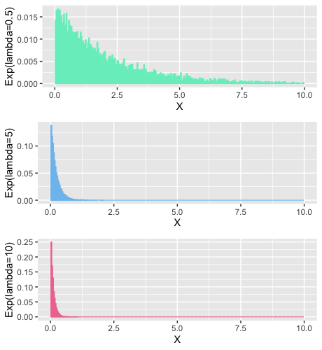
Intuitively , by the looks of it , we can infer that if some events are happening at a fast rate [large $\lambda$], its going to be exponentially rare that you will get to see the next event after a very long time [high value of t will have exponentially diminishing probabilities]
Mean
\[\begin{align} \mu &=E[X] \\&=\int\limits_{0}^{\infty}t\lambda e^{-\lambda t}dt \end{align}\]Remember integration by parts ? Good for you if you said yes. I don’t . So here is a reminder for all of us
\[\int u (\frac{dv}{dt})dt =uv -\int v \frac{du}{dt}dt\]In our expression earlier
\[\begin{align} u &= t \\\& \ \ v&=-\frac{e^{-\lambda t}}{\lambda} \end{align}\]so we can rewrite that expression using integration by parts formula
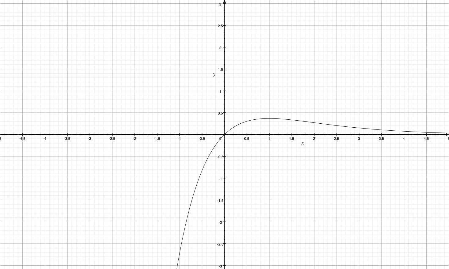
\[\begin{align} \mu &=\lambda\Big[-\frac{te^{-\lambda t}}{\lambda}\Biggr|_{0}^{\infty} +\int\limits_{0}^{\infty}\frac{e^{-\lambda t}}{\lambda}dt\Big] \end{align}\]Easiest and very intuitive way to understand, that expression $te^{-\lambda t}$ goes to 0 as $t \to \infty$; is to look at its plot
so ,
\[\begin{align} \mu &=\lambda \int\limits_{0}^{\infty}\frac{e^{-\lambda t}}{\lambda}dt \\&=\int\limits_{0}^{\infty}{e^{-\lambda t}}dt \\&=\frac{1}{\lambda} \end{align}\]Variance
\[\begin{align} E[X^2]&=\int\limits_{0}^{\infty}t^2\lambda e^{-\lambda t}dt \end{align}\]now here
\[\begin{align} u &= t^2 \\\& \ \ v&=-\frac{e^{-\lambda t}}{\lambda} \end{align}\]so,
\[\begin{align} E[X^2]&=\int\limits_{0}^{\infty}t^2\lambda e^{-\lambda t}dt \\&=\lambda\Big[-\frac{t^2e^{-\lambda t}}{\lambda}\Biggr|_{0}^{\infty} +\int\limits_{0}^{\infty}\frac{te^{-\lambda t}}{\lambda}dt\Big] \end{align}\]Graph for $t^2e^{-\lambda t}$ looks like this
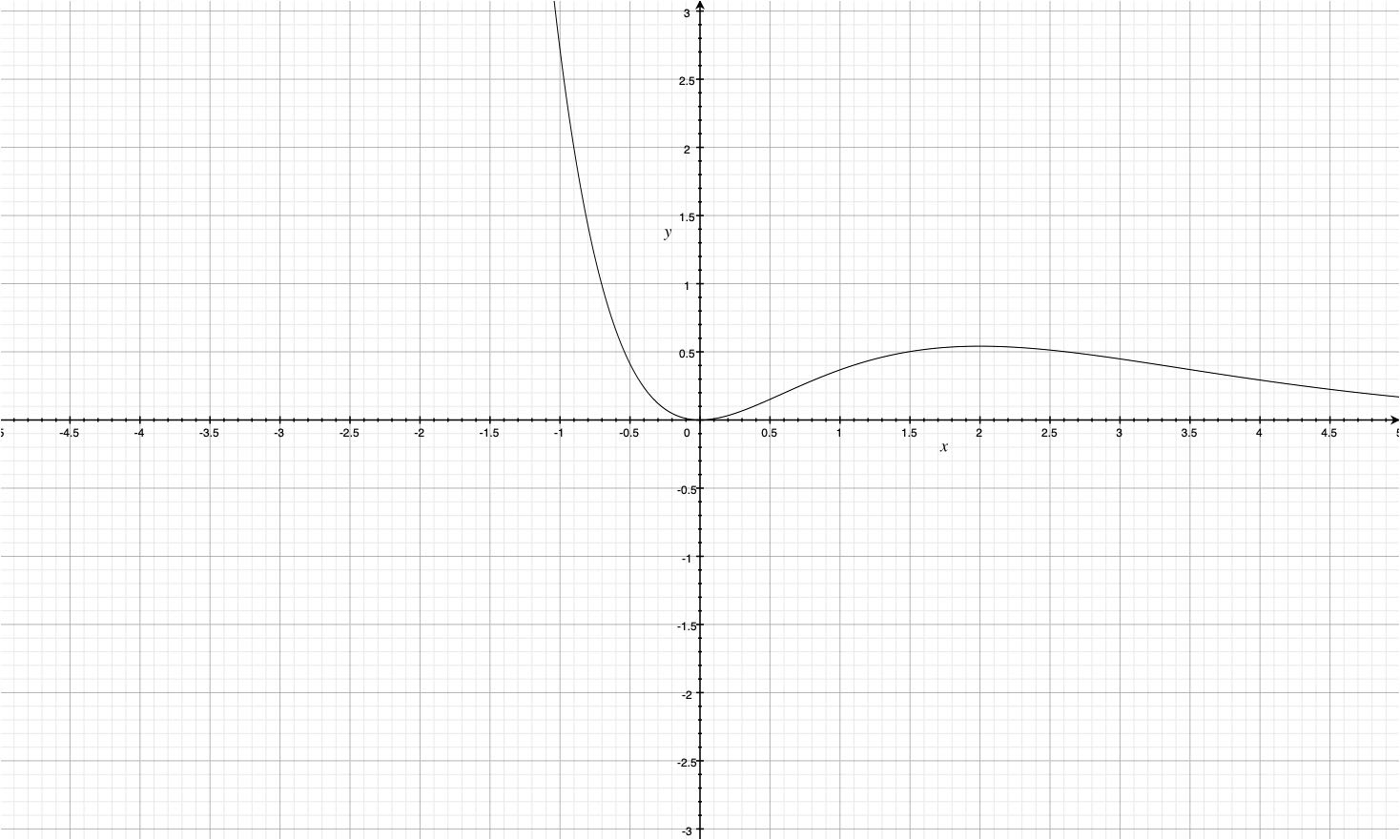
Clearly the first term in the expression above is going to be simply 0 again.
\[\begin{align} E[X^2]&=\int\limits_{0}^{\infty}t^2\lambda e^{-\lambda t}dt \\&=\lambda\Big[-\frac{t^2e^{-\lambda t}}{\lambda}\Biggr|_{0}^{\infty} +2\int\limits_{0}^{\infty}\frac{te^{-\lambda t}}{\lambda}dt\Big] \\&=2\int\limits_{0}^{\infty}{te^{-\lambda t}}dt \\&=\frac{2}{\lambda^2} \end{align}\]using this for variance
\[Var(X)=\frac{2}{\lambda^2}-\frac{1}{\lambda^2}=\frac{1}{\lambda^2}\]What does it look like
An example
Chef takes 5 minutes to make a burger . Whats the probability that chef will take 3 to 4 minutes to cook the next burger . You have all the tools at your disposal . Do it yourself .
What Next?
- Geometric, Negative Binomial , Hypergeometric
- Beta, Gamma, Weibull, Double Exponential
- Normal, Cauchy, Chi-Squared, t, F
Part 2 coming soon!
– Lalit Sachan [https://www.linkedin.com/in/lalitsachan/]