Feature Engineering in Machine Learning
09 Jul 2019
For a good time I believed that you can’t really give a long talk on feature engineering which will be relevant across multiple problem spaces. This belief originated from having seen people; calling problem specific special treatment of data; feature engineering . However , over the years I have unconsciously gathered pretty standard ways of treating different kind of features which are applicable irrespective of the kind of problem that you are working with. This of course doesn’t mean that there is no problem specific feature engineering , it simply implies that; you CAN have a good length discussion on generic feature engineering which applies well across different problems .
Sequence of different tips and tricks mentioned here doesn’t hold much meaning . I am simply writing/coding away things as and when I recall them here .
1. How to represent cyclic features
An intuitive example of such data columns are months or weekday numbers. Problem with simply giving them numbers is that the representation doesn’t really make sense . Why ?
Lets have a look :
| Month | Coded_Value |
|---|---|
| January | 1 |
| February | 2 |
| March | 3 |
| April | 4 |
| May | 5 |
| June | 6 |
| July | 7 |
| August | 8 |
| September | 9 |
| October | 10 |
| November | 11 |
| December | 12 |
December isn’t really (12-1=11) months away from January. The next guy is January, they are just 1 month apart. Their numerical coding which we intend to use as a simple numeric column , doesn’t represent the same information.
A simple trick , in such cases of cyclical data is to use cyclical functions for encoding the values.
\[\text{months_sin} = sin(\frac{2*\pi*Months}{12})\]In general this will be :
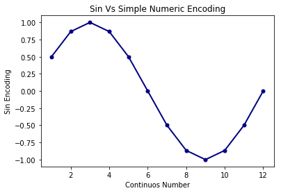
\[\text{x_sin} = sin(\frac{2*\pi*x}{max(x)})\]There is still a slight issue, simple plot of transformed values will clarify .

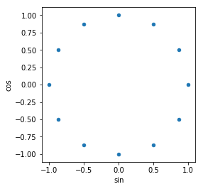
You can see that, now values start to turn up cyclically to have difference among them reducing as months near to end of year. The issue that I was talking about this approach , will become apparent if you look at values of month 2 and 4 . They have same values . The way to counter this is to use two cyclical functions ; both sin and cos. Any cyclic numeric column will be encoded as two columns, sin and cos transformations like this :
They look truly cyclic now. All the values in 2 dimensions are different and retain distances among them as per their cyclic nature. :

Here is a quick function for the same :
def code_cyclic_features(data,columns,drop_cols=True):
  for col in columns:
    max_val=max(data[col])

    data[col+'_sin']=np.sin(2*np.pi*data[col]/max_val)
    data[col+'_cos']=np.cos(2*np.pi*data[col]/max_val)

    if drop_cols:
      del data[col]
  return data
2. Coding Categorical Features as dummies/flags
Ignoring the discussion where you can convert the categorical feature to some numeric representation without changing the sense of information .
Everybody starts coding categorical columns by creating n-1 dummies for n categories . However we should keep in mind that if any category doesn’t have enough observations/data, we won’t be able to extract consistent/reliable patterns from it. It’s a common practice to ignore such categories. You have to decide a frequency cutoff. There isn’t much point in searching the depths of internet to find a good value for this cutoff. Keep the tradeoff in mind , higher cutoff will lead to information loss and lower cutoff will lead to data explosion and overfitting.
Here is a quick python function which will enable you to create dummies with frequency cutoff.
def code_categorical_to_dummies(data,columns,frequency_cutoff=100):

    for col in columns:
        freq_table=data[col].value_counts(dropna=False)
        cats=freq_table.index[freq_table>frequency_cutoff][:-1]
        for cat in cats:
            data[col+'_'+cat]=(data[col]==cat).astype(int)

        del data[col]


    return data
3. Categorical Embeddings
Even when you use frequency cutoff , sometimes creating dummies results in data explosion as all of the categories might have good number of observation. Consider a data which has 11 columns where 10 are numeric and 11th column has 50 eligible categories . You’ll end up with 60 columns in the data. This could be a problem if you further decide to build a randomforest or gbm family models. You’ll decide the max_features parameter to be some random subset of these 60 columns in your data. By sheer number, the flag variables coming from a single column will be selected a lot more and , 10 numeric columns don’t get enough exposure due to inbuilt nature of the algorithm. We’d like to represent these flag variables at much lower dimensions than creating 50 separate columns in this scenario.
What comes to your rescue is embedding derived from neural networks which work as auto encoders . Here is an example in code which will help you in understanding the concept .
file = r'/Users/lalitsachan/Dropbox/0.0 Data/loans data.csv'
data=pd.read_csv(file)
data['State'].nunique()
47
Column State here has 47 unique values . We can create dummies but that will lead to having 47 one hot encoded columns . Lets see how we can come up with model driven embeddings for this column and bring down the dimension for the same .
dummy_data=pd.get_dummies(data['State'],prefix='State')
dummy_data.shape[1]
47
We’ll take the columns as our response as well. The network that we’ll be building [ an autoencoder] will be solving a pseudo problem. Its job is to take this one hot encoded representation [ dummy_data] and spit out the same values as the outcome. I call it a pseudo problem to solve because i am not really interested in the model which takes the input and spits it out as outcome perfectly. What is actually of interest to me is the compression that the input goes through in the intermediate layers of this model. Goal to build this pseudo network well is to ensure that this compression is not leading to information loss, that can only be said, if outcome of the network matches with the input.
y=dummy_data
from keras.models import Model,Sequential
from keras.layers import Dense,Input

embedding_dim=3
inputs=Input(shape=(dummy_data.shape[1],))
dense1=Dense(20,activation='relu')(inputs)
embedded_output=Dense(embedding_dim)(dense1)
outputs=Dense(dummy_data.shape[1],activation='softmax')(embedded_output)
model=Model(inputs=inputs,outputs=outputs)

embedder=Model(inputs=inputs,outputs=embedded_output)
We are going to use output of embedder as our transformed data. Embedding is being driven by predicting the response .
model.compile(optimizer='adam',loss='categorical_crossentropy',metrics=['accuracy'])
model.fit(dummy_data,y,epochs=150,batch_size=100)
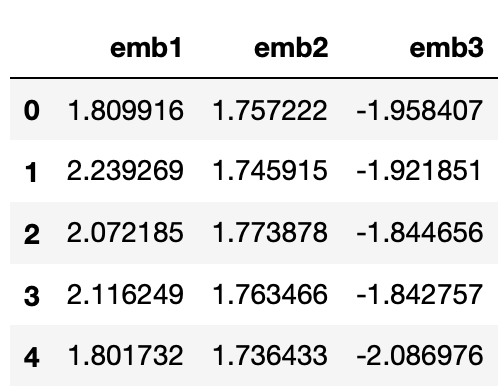
Once this is done , we can use embedder to get out transformed data, new low dimensional representation of 47 one hot encoded columns
low_dim=pd.DataFrame(embedder.predict(dummy_data),columns=['emb1','emb2','emb3'])
low_dim.head()

We can use the same trained embedder for test/val data as well.
4. Feature Selection using feature importance
Important Update :While this idea is good and sound. Implementation of feature importance in R/Python is not proper . And you should be cautious about using the same . You'll find more details here :
https://explained.ai/rf-importance/
It’s a common feature of many tree based ensemble method (both bagging and boosting), feature importance , which can be used for quick feature selection . But many sources failed to mention, where to draw the line. What level of feature importance should be set as cutoff , below which you can drop all the columns from further considerations .
Truth is , people don’t mention this because as such there is no fixed cutoff. And meaning of numeric value of feature importance can be data dependent. However a neat little trick can be used every time. You can add a random noise column as one of the features . Any column which gets its feature importance value below that, can be considered doing worse than white noise , which we know is not related to data and hence can be dropped.
Here is a quick example using one of the pre loaded datasets in sk-learn.
from sklearn.datasets import load_boston
boston=load_boston()

X=pd.DataFrame(boston.data,columns=boston.feature_names)
y=boston.target
We’ll add random noise to the data
X['white_noise']=np.random.random(size=(X.shape[0]))
Now lets build a quick random Forest model and check feature importance to see which features we can safely drop before further more detailed experiments with the data
from sklearn.ensemble import RandomForestRegressor
rf=RandomForestRegressor(n_estimators=200)
rf.fit(X,y)
imp_data=pd.DataFrame({'imp':rf.feature_importances_,'cols':X.columns})
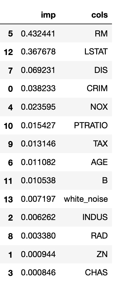
imp_data.sort_values('imp',ascending=False)

We can safely say that , we can drop columns INDUS, RAD, ZN, CHAS in context of predicting the target for this problem .
5. Ratio Features
As we move towards complex algorithms , need for manual feature creation goes down as many of the transformations can be learned by the algorithms of sufficient complexity ( Neural Networks , Boosting Machines ). Example of such transformations can be features created as interaction variables , log transformations or polynomials of original features in the data.
However ratio features are the ones which different algorithms are consistently bad at emulating . If you think that in context of the business problem that you are trying to solve; ratio of features in data can play definitive role then you should create them manually; instead of relying on any algorithm to extract that pattern.
A simple example of ratio variable can be utilisation of credit cards [ratio between expense and limit]
You can find a detailed discussion about what kind of feature transformation different algorithms can emulate and what they can not : here
Few notes on the takeaways/followups .
- This is not an exhaustive list by any means. I discussed few things which I see; are not commonly discussed or are generally looked over. I’ll make additions if I recall something else.
- Whenever I discussed one of the tricks, I skimmed over other details. For example , when we were talking about categorical embeddings , we can very well first ignore categories which have low frequencies , create dummies for the rest and then go for categorical embeddings .
- Feel free to let me know if you’d like me to add some discussion as part/addition to the list above.
