07 Sep 2020

Part1
In first part of this series we saw many distributions which arise as some variations of collection of Bernoulli trials ; binomial distribution . I mention this to make you realise that distributions are nothing but tools to make probability calculations easy and handy . The same way you could probably derive the derivative of $\sin{x}$ to be $\cos{x}$ using the first principle every time you needed it ; but its far easier to simply use the pre-derived formulae . In essence , distributions are pre-done complex probability calculations which can then be used to do many useful things; without starting from scratch .
We’ll continue our journey to find other distributions arising from variations of binomial distribution. Starting with Geometric Distribution
Geometric Distribution
Imagine that there is 10% chance that you can hit the bulls eye in a game of darts [ or make a profit on a share buy, sadly the same thing these days ]. Whats the probability that you’ll go without hitting the bulls eye for 6 consecutive throws , before eventually hitting the prize shot . Thats geometric distribution for you. Probability of $(K-1)$ consecutive failures before you see success in the $K^{th}$ trial .
\[P(x=K) = q^{k-1}p\]
As we have been doing for other distributions , we’d like to calculate the mean and variance for geometric distribution also. As we have done earlier , before we jump into doing that, we’ll derive some tricky maths results and use them later.
We will start with the expression for sum of an infitite geometric series .
\[\begin{align}
\sum\limits_{k=0}^\infty b^k =\frac{1}{1-b}
\end{align}\]
Lets differentiate on both sides $w.r.t. b$ once :
\[\begin{align}
& \ \sum\limits_{k=1}^\infty kb^{k-1} =\frac{1}{(1-b)^2}
\end{align}\]
We’ll do this once more after multiplying both sides by $b$ once :
\[\begin{align}
& \ \sum\limits_{k=1}^\infty kb^{k} =\frac{b}{(1-b)^2}
\\ & \ \sum\limits_{k=1}^\infty k^2b^{k-1} =\frac{1}{(1-b)^2}+\frac{2b}{(1-b)^3}
\\ & \ \sum\limits_{k=1}^\infty k^2b^{k-1} =\frac{1+b}{(1-b)^3}
\end{align}\]
in short, two results that we derived are :
- $\sum\limits_{k=1}^\infty k b^{k-1} =\frac{1}{(1-b)^2}$
- $\sum\limits_{k=1}^\infty k^2 b^{k-1}=\frac{(1+b)}{(1-b)^3}$
mean
\[\begin{align}
\mu &= E[X]
\\&= \sum\limits_{k=1}^\infty k q^{k-1}p
\\&=\frac{p}{(1-q)^2}=\frac{p}{p^2}=\frac{1}{p}
\end{align}\]
This simply implies that if you have 15% chance to hit the bulls eye, on an average ; it will take you $\frac{1}{.15} \sim 7$ attempts to get that shot .
Variance
\[\begin{align}
E[X^2]&=\sum\limits_{k=1}^\infty k^2 q^{k-1}p
\\&= \frac{p(1+q)}{(1-q)^3}=\frac{1+q}{p^2}
\end{align}\]
\[\begin{align}
Var(X) &= E[X^2]-(E[X])^2
\\&=\frac{1+q}{p^2}-\frac{1}{p^2}=\frac{q}{p^2}
\end{align}\]
and the variance in this number , number of attempts that it takes people to get first success is going to be $\frac{0.85}{0.15^2} \sim 37$ , which is a huge number especially in comparison to the average number of trials it’s going to take. Insight that you should derive from here is that , for a low success task, don’t be deceived by a small average , be vary of the variance .
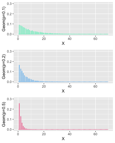
what does it look like
The only parameter this distribution has, is $p$ .

Notice that for low success scenarios , probability of early success is low , and the chance of getting success later, extends much farther in comparison to high success rate scenarios. Variance is also low for high success scenarios .
HyperGeometric Distribution
In the scenarios discussed so far, we have not considered the case of finite population . Consider this question, if a city of 10000 residents has 200 doctors . Whats the probability that out of 100 randomly selected citizens , 10 are doctors .
A generic formula to answer this question will consider, Population size = N, number of successes present in the population = M, Size of the sample being taken = n . then
\[P(X=x)=\frac{\binom{M}{x}*\binom{N-M}{n-x}}{\binom{N}{n}}\]
This is our hypergeometric distribution. note that there is a limit on value of $x$ and $n$ here , since the population is finite . $n\in [1,N]$ and $x \in [0,n]$ .
time for deriving maths results for using later
\[\begin{align}
r*\binom{n}{r}&=\frac{r * n!}{r!* (n-r)!}
\\ &=\frac {n*(n-1)!}{(r-1)!(n-1-(r-1))!}
\\&=n*\binom{n-1}{r-1}
\end{align}\]
mean
\[\begin{align}
E[X]&=\sum\limits_{x=1}^{n}\frac{x*\binom{M}{x}*\binom{N-M}{n-x}}{\binom{N}{n}}
\\ &=\sum\limits_{x=1}^{n}\frac{M*\binom{M-1}{x-1}*\binom{N-M}{n-x}}{\binom{N}{n}}
\\&=\sum\limits_{x=1}^{n}\frac{M*\binom{M-1}{x-1}*\binom{N-1-(M-1)}{n-1-(x-1)}}{\binom{N}{n}}
\\ &=\frac{M}{\binom{N}{n}}*\binom{N-1}{n-1}\sum\limits_{x=1}^{n}\frac{\binom{M-1}{x-1}*\binom{N-1-(M-1)}{n-1-(x-1)}}{\binom{N-1}{n-1}}
\end{align}\]
The expression written inside the summation here is another hypergeometric distribution with parameters $N-1$ , $M-1$ and $n-1$ . This pmf summed over all values of $x$ will simply be 1.
\[\begin{align}
E[X]&=\frac{M}{\binom{N}{n}}*\binom{N-1}{n-1}\sum\limits_{x=1}^{n}\frac{\binom{M-1}{x-1}*\binom{N-1-(M-1)}{n-1-(x-1)}}{\binom{N-1}{n-1}}
\\&=\frac{M}{\binom{N}{n}}*\binom{N-1}{n-1}
\\&=\frac{M*n!*(N-n)!}{N!}*\frac{(N-1)!}{(n-1)!(N-n)!}
\\&=\frac{M*n}{N}
\end{align}\]
Now if you think about it , $\frac{M}{N}$ is the probability of success and the result that you see above is simply $np$ , same as what we got for binomial distribution .
Variance
\[\begin{align}
E[X^2]&=\sum\limits_{x=1}^{n}\frac{x^2*\binom{M}{x}*\binom{N-M}{n-x}}{\binom{N}{n}}
\\ &= \sum\limits_{x=1}^{n}\frac{x*M*\binom{M-1}{x-1}*\binom{N-M}{n-x}}{\binom{N}{n}}
\\ &= \sum\limits_{x=1}^{n}\frac{(x-1+1)*M*\binom{M-1}{x-1}*\binom{N-M}{n-x}}{\binom{N}{n}}
\\&= \sum\limits_{x=1}^{n}\frac{(x-1)*M*\binom{M-1}{x-1}*\binom{N-M}{n-x}}{\binom{N}{n}}+\sum\limits_{x=1}^{n}\frac{M*\binom{M-1}{x-1}*\binom{N-M}{n-x}}{\binom{N}{n}}
\\&= \sum\limits_{x=1}^{n}\frac{M*(M-1)\binom{M-2}{x-2}*\binom{N-M}{n-x}}{\binom{N}{n}}
+\frac{M*\binom{N-1}{n-1}}{\binom{N}{n}}\sum\limits_{x=1}^{n}\frac{\binom{M-1}{x-1}*\binom{N-M}{n-x}}{\binom{N-1}{n-1}}
\\&= \frac{M*(M-1)*\binom{N-2}{n-2}}{\binom{N}{n}}\sum\limits_{x=1}^{n}\frac{\binom{M-2}{x-2}*\binom{N-2-(M-2)}{n-2-(x-2)}}{\binom{N-2}{n-2}}
+\frac{M*\binom{N-1}{n-1}}{\binom{N}{n}}\sum\limits_{x=1}^{n}\frac{\binom{M-1}{x-1}*\binom{N-1-(M-1)}{n-1-(x-1)}}{\binom{N-1}{n-1}}
\end{align}\]
The first summation is pmf of a hypergeometric distribution with parameters $N-2$,$M-2$,$n-2$ ;the second term is the same but with parameters $N-1$,$M-1$,$n-1$ . Both of them will sum up to 1 .
\[\begin{align}
E[X^2]&= \frac{M*(M-1)*\binom{N-2}{n-2}}{\binom{N}{n}}\sum\limits_{x=1}^{n}\frac{\binom{M-2}{x-2}*\binom{N-2-(M-2)}{n-2-(x-2)}}{\binom{N-2}{n-2}}
+\frac{M*\binom{N-1}{n-1}}{\binom{N}{n}}\sum\limits_{x=1}^{n}\frac{\binom{M-1}{x-1}*\binom{N-1-(M-1)}{n-1-(x-1)}}{\binom{N-1}{n-1}}
\\&=\frac{M*(M-1)*\binom{N-2}{n-2}}{\binom{N}{n}}
+\frac{M*\binom{N-1}{n-1}}{\binom{N}{n}}
\\&=\frac{M*(M-1)*(N-2)!n!(N-n)!}{(n-2)!(N-n)!N!}+\frac{M*(N-1)!n!(N-n)!}{N!(n-1)!(N-n)!}
\\&=\frac{M*(M-1)*n*(n-1)}{N*(N-1)}+\frac{M*n}{N}
\\&=\frac{M*n}{N}\Big[\frac{(M-1)*(n-1)}{N-1}+1\Big]
\end{align}\]
Now that we have managed to get this , lets go to the variance
\[\begin{align}
Var(X)&=E[X^2]-(E[X])^2
\\&=\frac{M*n}{N}\Big[\frac{(M-1)*(n-1)}{N-1}+1\Big] -\frac{M^2*n^2}{N^2}
\\&=\frac{M*n}{N}\Big[\frac{(M-1)*(n-1)}{N-1}+1-\frac{M*n}{N}\Big]
\\&=\frac{M*n}{N}\Big[\frac{M*n*N-M*N-n*N+N+N^2-N-M*n*N+M*n}{N*(N-1)}\Big]
\\&=\frac{M*n}{N}\Big[\frac{-M*N-n*N+N^2+M*n}{N*(N-1)}\Big]
\\&=\frac{M*n}{N}\Big[\frac{N*(N-n)-M*(N-n)}{N*(N-1)}\Big]
\\&=\frac{M*n}{N}\Big[\frac{(N-M)*(N-n)}{N*(N-1)}\Big]
\\&=n*\frac{M}{N}*\Big(1-\frac{M}{N}\Big)\frac{(N-n)}{(N-1)}
\end{align}\]
This again is close to $npq$ ; which was the variance of binomial distribution . [considering $\frac{M}{N}=p$], however it comes with correction factor $\frac{N-n}{N-1}$; also known as finite population correction factor for binomial distribution .
Another way to differentiate between binomial distribution and hypergeometric distribution is to look at hypergeometric distribution as the result of sampling without replacement and binomial distribution to be sampling with replacement [letting go of the constraints on population size].
I am skipping the what does it look like section here as the visuals are mostly going to be like binomial distribution.
Negative Binomial Distribution
Recall that, binomial variable was defined as number of successes you might get to see in fixed number of trials . What if we now want to consider a scenario where number of successes are fixed and we would like to know, how many trials it will take to reach there .
\[P(X=x)=\binom{x-1}{r-1}*p^r*q^{(x-r)}\]
There is another more common expression for this distribution; which makes further calculations rather convenient and thats the expression where the distribution derives its name from .Instead of looking at number of trials required [say $x$] to reach $r$ successes, we’ll use number of failures [say $y$] before $r^{th}$ success . This relationship holds between this $x$ and $y$ .
\[y=x-r\]
and pmf for this variable is given by
\[P(Y=y)=\binom{y+r-1}{y}*p^r*q^{y}\]
The binomial coefficient that you see here appears in negative binomial expressions , that is where the name comes from. Next we are going to derive some maths to make our job easy later while calculating mean and variance of these distributions .
\[\begin{align}
\binom{y+r-1}{y}&=\frac{(y+r-1)(y+r-2)(y+r-3)\cdots r(r-1)(r-2)\cdots3*2*1}{y!(r-1)!}
\\&=\frac{(y+r-1)(y+r-2)(y+r-3)\cdots r}{y!}
\\&=(-1)^y\frac{(-r)(-r-1)\cdots(-r-(y-1))}{y!}
\\&=(-1)^y*\binom{-r}{y}
\end{align}\]
Next bit we will start with Taylor’s expansion of a function :
\[f(x)=\sum_{k=0}^\infty f^{(k)}(a)\frac{(x-a)^k}{k!}\]
Where $ f^{(k)} $ is $ k^{th} $ derivative of $f$ and $x\to a$. Now consider $a=0$ . That makes the above expression a maclaurin series [ putting the name here , so that you can go explore more if you are interested] . Since we are considering $a$ to be $0$ here , this will work for $x \to 0$ , or $\lvert x \rvert <1 $ .
\[f(x)=\sum_{k=0}^\infty f^{(k)}(0)\frac{x^k}{k!}\]
Lets consider a special function to use this for :
\[\begin{align}
& 1. \ f(x)=(1-x)^{-r}
\\& 2. \ f^{(k)}(x) =(-1)^k (-r)*(-r-1)*(-r-2)\cdots*(-r-(k-1))(1-x)^{(-r-k)}
\\& 3. \ f^{(k)}(0) =(-1)^k (-r)*(-r-1)*(-r-2)\cdots*(-r-(k-1))
\end{align}\]
Using the maclaurin series given above we can write :
\[\begin{align}
(1-x)^{-r}&=\sum_{k=0}^\infty (-1)^k \frac{(-r)*(-r-1)*(-r-2)\cdots*(-r-(k-1))}{k!}*x^k
\\ &=\sum\limits_{k=0}^\infty (-1)^k *\binom{-r}{k}*x^k
\end{align}\]
Lets differentiate this $w.r.t. \ x$ once on both sides
\[\begin{align}
& \ r(1-x)^{-r-1}=\sum\limits_{k=0}^\infty (-1)^k *k*\binom{-r}{k}*x^{k-1}
\\ & \ rx(1-x)^{-r-1}=\sum\limits_{k=0}^\infty (-1)^k *k*\binom{-r}{k}*x^{k}
\end{align}\]
Once more :
\[\begin{align}
& \ r(1-x)^{-r-1}+rx(r+1)(1-x)^{-r-2}=\sum\limits_{k=0}^\infty (-1)^k *k^2*\binom{-r}{k}*x^{k-1}
\\& \ rx(1-x)^{-r-1}+rx^2(r+1)(1-x)^{-r-2}=\sum\limits_{k=0}^\infty (-1)^k *k^2*\binom{-r}{k}*x^{k}
\\& \ rx(1-x+rx+x)(1-x)^{-r-2}=\sum\limits_{k=0}^\infty (-1)^k *k^2*\binom{-r}{k}*x^{k}
\\& \ rx(rx+1)(1-x)^{-r-2}=\sum\limits_{k=0}^\infty (-1)^k *k^2*\binom{-r}{k}*x^{k}
\end{align}\]
Summarising results that we will be using :
\[\begin{align}
& 1. \ \binom{y+r-1}{y} = (-1)^y*\binom{-r}{y}
\\ & 2. \ (1-x)^{-r} = \sum\limits_{k=0}^\infty (-1)^k *\binom{-r}{k}*x^k
\\ & 3. \ \sum\limits_{k=0}^\infty (-1)^k *k*\binom{-r}{k}*x^{k}=rx(1-x)^{-r-1}
\\ & 4. \ \sum\limits_{k=0}^\infty (-1)^k *k^2*\binom{-r}{k}*x^{k}=(rx+1)rx(1-x)^{-r-2}
\end{align}\]
Mean
\[\begin{align}
E[Y]&=\sum\limits_{y=0}^\infty y*\binom{y+r-1}{y}*p^r*q^{y}
\\&=\sum\limits_{y=0}^\infty (-1)^{y}*y*\binom{-r}{y}*p^r*q^{y}
\\&=p^r\sum\limits_{y=0}^\infty (-1)^{y}*y*\binom{-r}{y}*q^{y}
\\&=p^r*r*q(1-q)^{-r-1}=p^r*r*q*p^{-r-1}=\frac{rq}{p}
\end{align}\]
If you need to hit the bullseye at-least 3 times in the same night to appear on the hall of fame board of the bar , how many times on an average you need to try throwing darts; given that the probability of you hitting the bulls eye is $\frac{1}{10}$ . Using the result above , the answer comes to be $\frac{3*\frac{9}{10}}{\frac{1}{10}} = 42$ , that is average number of failures , before the 3rd success, meaning $42+3=45$ trials , before you make it to the hall of fame. Woah, you better get really good at darts , or just be patients , or may be not so ambitious otherwise . Life has other things to offer, you just need to look beyond the ….Bulls eye.
Variance
\[\begin{align}
E[Y^2]&=\sum\limits_{y=0}^\infty y^2*\binom{y+r-1}{y}*p^r*q^{y}
\\&=p^r\sum\limits_{y=0}^\infty y^2*\binom{y+r-1}{y}*q^{y}
\\&=p^r\sum\limits_{y=0}^\infty (-1)^y*y^2*\binom{-r}{y}*q^{y}
\\&=p^r(rq+1)*r*q*p^{-r-2}
\\&=(rq+1)\frac{rq}{p^2}
\end{align}\]
\[\begin{align}
Var[Y]&=E[Y^2]-(E[Y])^2
\\&=(rq+1)\frac{rq}{p^2}-\frac{r^2q^2}{p^2}
\\&=\frac{rq}{p^2}(rq+1-rq)=\frac{rq}{p^2}
\end{align}\]
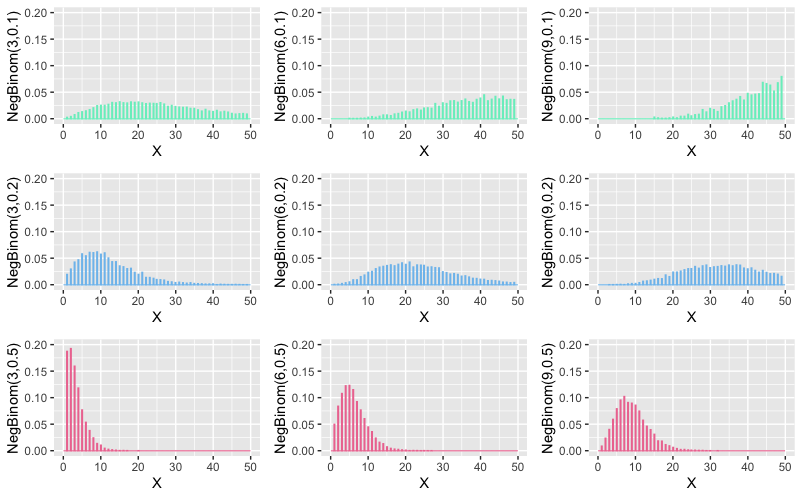
what does it look like

See, how low success rate scenarios end up being very flat , positively skewed and fat tailed , for low number of success. And as number of successes start to go up, distribution for high success scenarios also start to shift to right, but much slower.
Concluding this post
So far our discussions on this series have been mostly on discrete distributions [Exponential distribution , briefly popped up towards the end of the last post]. In the next post, we’ll be going to unravel mysteries of continuous distributions. Where they come from, how can we understand them; both as limiting cases of discrete distributions, as well as relate them to real life continuous data.
If you haven’t read the first part , here it is
Part1
07 Jul 2020

All the distributions that we will discuss, can be categorised into two broad groups : Discrete and Continuous .
- Discrete distributions pertain to data which contains discrete outcomes [Integers] as their values. E.g. Number of people on the train , Count of bees in an honeycomb . [Imagine the horror of seeing three and quarter of a person getting off the train!]
- Continuous distributions on the other hand have values which can take values in decimals . E.g. Weight of students in a class, Length of trees in a forest [Number of people in a zombie movie?]
We’ll start our discussion with a very simple and intuitive distribution known as uniform distribution . In that discussion we will also learn about defining and calculating mean and variance as Expectation.
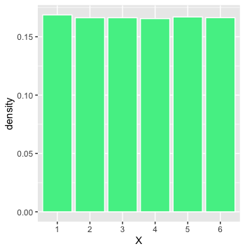
Uniform distribution is where each value in the distribution has equal probability of occurrence . If we had to come up with a general expression for probability of occurrence of each value in the uniform distribution, we can write .
\[P(X=x) = \frac{1}{n}\]
Where n is the number of values in the range of the distribution. A classic example which produces uniform distribution is throwing a fair dice. 🎲
Each throw might result in any of the $ {1,2,3,4,5,6}$ on the top face with equal probability . So in this case
\[P(X=x)=\frac{1}{6} \ \ \forall \ x \in \{1,2,3,4,5,6\}\]
Expectation
Consider a gambling party where the host has gone bonkers and is asking guests to throw a dice and collect as much money as the number which shows on the face of the dice. However if you get 1 , you have to give $ 10 to the host.On an Average how much money the host is going to make [or lose] on each player.
We can start by assuming there are 72 [ the number doesn’t really matter ] people in the party . Since the dice is fair; we can assume that each of ${1,2,3,4,5,6}$ will be obtained by 12 guests.
- So the money lost by host $ {=12X6 + 12X 5 + 12X4 +12X3 +12X2 = $ 240} $
- money gained by host $=12X10 = $120$
- Overall money lost by host $= 240 - 120 = $120$
- Money lost per player $\frac{$120}{72}=$1.67$
A simpler way of doing this will be to multiply probability of each outcome with the outcome and sum them.
Average gain
\(=-6*\frac{1}{6}-5*\frac{1}{6}-4*\frac{1}{6}-3**\frac{1}{6}-2*\frac{1}{6}+10*\frac{1}{6}=\$1.67\)$
This is also known as expected value of a distribution [or mean]. A formal expression for the same will be
\[\mu = E[X] = \sum xP(X=x)\]
Let’s calculate mean of uniform distribution like this . Say distribution takes integer values in the interval $[a,b]$ with $n$ values in it.
[$b = a + (n-1)$], Since $b$ is the $n^{th}$ element .
\[\begin{align}
\mu & = E[X]
\\ & =[a+(a+1)+(a+2).....+b]*\frac{1}{n}
\\ & = [n*a + (1+2+3....n-1)]*\frac{1}{n}
\\ & = [n*a + (n-1)*\frac{n}{2} ]*\frac{1}{n}
\\ & =\frac{2a+n-1}{2}
\\ & =\frac{a+a+n-1}{2}
\\ & =\frac{a+b}{2}
\end{align}\]
Before we proceed further I will mention here few algebraic properties of expectation which are easy to derive; so I am going to put them here without extensive proof.
- $E[g(X)] = \sum g(x)P(X=x)$
- $E[const]=const$
- $E(aX+b) = aE(X)+b$
Variance of a distribution is defined as expectation of $(X-\mu)^2$ . [remember variance was mean of squared deviations from the mean]
\[\begin{align}
Var(X)&=E[(X-\mu)^2]
\\ &= E[X^2 + \mu^2 - 2\mu X]
\\ &= E[X^2]+\mu^2-2\mu E[X]
\\&= E[X^2]-\mu^2
\\&=E[X^2]-(E[X])^2
\end{align}\]
Lets calculate variance of uniform distribution with this
\[\begin{align}
E(X^2)&=[a^2+(a+1)^2+.......(a+n-1)^2]*\frac{1}{n}
\\ & = [n*a^2 + (1+2^2+3^2+......(n-1)^2) - 2*a(1+2+3....n-1)]*\frac{1}{n}
\\ & = [n*a^2 + \frac{(n-1)n(2n-1)}{6}-2*a*\frac{(n-1)(n)}{2}]*\frac{1}{n}
\\ & = a^2 + \frac{(b-a)(b-a+1)(2b-2a+1)}{6}-a(b-a)(b-a+1)
\\ &\;\;\vdots
\\ Var(X) & = E(X^2)-[E(X)]^2
\\ & = \frac{(b-a)^2}{12}
\end{align}\]
I have skipped some algebraic gymnastic there. Do it yourself if it rubbed your marbles the wrong way.
For continuous distributions ; if the pdf is given as $f(x)$ then
Key Takeaways
About expectations :
- $E[X]=\sum xP(X=x) = \int xf(x)dx$
- $Var(X)=E[X^2]-(E[X])^2$
About discrete uniform distribution :
- $P(X=x)=\frac{1}{n} \forall x \in {a,a+1,…b} \ with \ n \ elements$
- $\mu = E(X) = \frac{(a+b)}{2}$
- $Var(X) = \frac{(b-a)^2}{12}$
What does it look like

Bernoulli’s Distribution [Discrete]
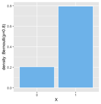
We get a call on our phone , we receive it or we don’t . We are driving on the road , we reach home safely or we die [ well that went from 0 to dead pretty fast] . Life is full of transactions which have two outcomes . 0/1 , failure/success, accept/decline and so on.
And each of these outcomes have some associated probability . Like there is 90% chance of an advice being solid gold if given by an old dude while peeling an apple with a pocket knife and eating pieces right off the blade . Oddly specific but relatable.
Formally we write :
\[P(X=x) =
\begin{cases}
p & \text{ if x =1} \\
q & \text{ if x =0, where q =1-p}
\end{cases}\]
Mean
\[\begin{align}
\mu &= E[X]
\\ &= 1 * p + 0*q
\\ & =p
\end{align}\]
Variance
\[\begin{align}
E[X^2] & = 1^2 * p + 0^2*q
\\&=p
\\Var(X) &= E[X^2]-[E[X]]^2
\\&=p-p^2=p*(1-p)
\\&=pq
\end{align}\]
What does it look like

Life is nothing but a sequence of countless Bernoulli Trials .
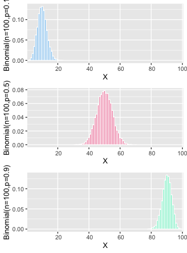
Binomial Distribution [Discrete]
During the pandemic lockdown, you have learnt to make absolutely killer cocktails. Probability of a person getting shitfaced drunk on the cocktail is $p$ . Let’s say $n$ people attended your party once the lockdown opens , what are the chances that $x$ of them will have no memory of what happened that night ?
$x$ is just number of guests . It can be made up of any $x$ guests out of $n$ . We can chose $x$ guests out of $n$ in ${}^{n}C_{x}$ ways.
\[\begin{align}
{}^{n}C_{x} &= \frac{!n}{!x!(n-x)}
\\
\\ \text{given }!n &= n*n(n-1)\cdots2*1
\end{align}\]
formally we can write [considering $q=1-p$]
\[P(X=x) = {}^{n}C_{x} * p^x *q^{n-x}\]
Before we get down to calculating mean and variance , let’s get done with some mean looking maths involving binomial coefficients .
We know that $(a+b)^n$ can be expanded using following expression involving binomial coefficients .
\[(a+b)^n = \sum\limits_{r=0}^{n}{}^{n}C_{r}a^r b^{n-r}\]
Now to the mean maths; we are going to derive some results which will come in handy later.
\[\begin{align}
\sum\limits_{r=0}^{n} r *{}^{n}C_{r} * a^r *b^{n-r} &= a* \sum\limits_{r=0}^{n} r *{}^{n}C_{r} * a^{r-1} *b^{n-r}
\\&= a*\frac{d}{da}[\sum\limits_{r=0}^{n} {}^{n}C_{r} * a^r *b^{n-r}]
\\&=a*\frac{d}{da}[(a+b)^n]
\\&=na(a+b)^{n-1}
\\ \sum\limits_{r=0}^{n} r^2 *{}^{n}C_{r} * a^r *b^{n-r} &= \sum\limits_{r=0}^{n} r(r-1) *{}^{n}C_{r} * a^r *b^{n-r}+\sum\limits_{r=0}^{n} r *{}^{n}C_{r} * a^r *b^{n-r}
\\&=a^2\sum\limits_{r=0}^{n} r(r-1) *{}^{n}C_{r} * a^{r-2} *b^{n-r}+na(a+b)^{n-1}
\\&=a^2*\frac{d}{da}[\sum\limits_{r=0}^{n} r *{}^{n}C_{r} * a^{r-1} *b^{n-r}]+na(a+b)^{n-1}
\\&=a^2*\frac{d}{da}[\frac{d}{da}[\sum\limits_{r=0}^{n} {}^{n}C_{r} * a^{r} *b^{n-r}]]+na(a+b)^{n-1}
\\&=a^2*\frac{d}{da}[\frac{d}{da}[(a+b)^n]]+na(a+b)^{n-1}
\\&=n(n-1)a^2(a+b)^{n-2}+na(a+b)^{n-1}
\end{align}\]
Mean
\[\begin{align}
\mu &= E[X]
\\ &= \sum\limits_{x=0}^{n} x *{}^{n}C_{x} * p^x *q^{n-x}
\\&=np(p+q)^{n-1}
\\&=np \ \ \ [\text{since $p+q=1$}]
\end{align}\]
Variance
\[\begin{align}
E[X^2] &=\sum\limits_{r=0}^{n} x^2 *{}^{n}C_{x} * p^x *q^{n-x}
\\&=n(n-1)p^2(p+q)^{n-2}+np(p+q)^{n-1}
\\&=n(n-1)p^2+np
\\Var(X) &=E[X^2]-[E[X]]^2
\\&=n(n-1)p^2+np-n^2p^2
\\&=np(1-p)
\\&=npq
\end{align}\]
What does it look like

CDF [cumulative density function]
Many at times , probability of an instance is not very useful. And it’s better to have a look at probability of an interval instead . This can be calculated as difference between cumulative probabilities which are defined as follows [given that X takes values in the interval $[a,b]$]
- for discrete distribution $CDF = P(X\le x) = \sum\limits_{x=a}^{x}P(X=x)$
- for continuous distributions = $\int\limits_{a}^{x}f(x)dx$
An Example
for a large clinical trial where there were 1000 patients and probability of success was 20% . answer following questions [I have added R codes, wherever needed]
- whats the expected number of cured patients = np = 1000*0.2=200
- whats the expected standard deviation across multiple such clinical trials $= \sqrt{npq}=\sqrt{1000X0.2X0.8} =12.6$
# whats the probability that 200 of the patients will be cured
dbinom(200,1000,0.2)

# whats the probability that upto 200 patients will be cured [use functions for cdf]
pbinom(200,1000,0.2)

# whats the probability that number of patients cured
# will be between 190 and 210 [use function for cdf]
pbinom(210,1000,0.2)-pbinom(190,1000,0.2)
I did not explicitly mention, but I hope you realised that Binomial Distribution is collection of Bernoulli trials . Where each individual outcome is from Bernoulli distribution. Binomial Distribution’s outcome is nothing but sum of the outcomes of those Bernoulli trials.
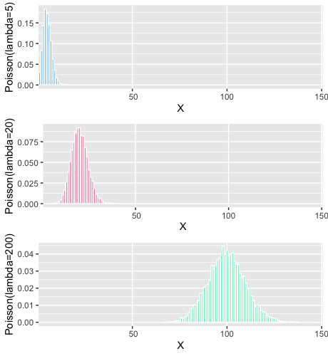
Poisson Distribution [Discrete]
You hear the unsavoury news that someone found an iron nail in their sausage and suddenly everyone in the group starts recounting similar experiences; and makes you feel as if this has become a very common phenomenon and world has gone to dogs and its a mistake to become a parent in these times and blah blah blah .
But if you take a step back and for a moment consider that; millions of sausages are consumed everyday and you rarely get to hear about someone really finding a nail in theirs. Mostly because, not finding a nail in your sausage is not NEWS, but finding a nail means; hell has finally frozen over. Same as a thousands of cars mundanely passing a town centre do not become talk of the town, but a single accident does.
I did not take this crazy sounding; sudden tangent in our discussion to play down the risk of nails or accident. The strange take aways that i want you to have from following news bite : ` there were 5 accidents last month in this traffic junction` are :
- We don’t know whats the probability of an individual vehicle passing the junction getting into an accident , but we do know that its pretty small despite the hullabaloo about the accidents
- We also know that thousands of vehicle must have passed through the junction which eventually resulted in these 5 accidents. But we don’t know the exact value of $n$ either.
So this month of 5 accidents was essentially a huge collection of Bernoulli trials with a very small probability of success. Basically this value 5 is coming from a Binomial distribution with very large $n$ and very small $p$
We’ll call this 5 accidents/month to be rate of events and denote it with symbol $\lambda$
\[\begin{align}
\lambda&=np
\\ p &= \frac{\lambda}{n}
\end{align}\]
Now with this information, someone asks you, can you tell me whats the probability that we’ll see $x$ accidents next month [given that flow of vehicles through the junction remains similar and other traffic conditions also remain unchanged]. Let’s try to answer that question in absence of information of both $n$ and $p$ . All that we have, is the rate $\lambda$ and hunch that $n$ is large and $p$ is small.
But it still is a binomial distribution . [well for now at-least , but we are going in for the kill boys!]
\[\begin{align}
\lim\limits_{n\to\infty} P(X=x) &= \lim\limits_{n\to\infty}{}^{n}C_{x} * p^x *q^{n-x}
\\&=\lim\limits_{n\to\infty}\frac{!n}{!x!(n-x)} * \Big(\frac{\lambda}{n}\Big)^{x}* \Big(1-\frac{\lambda}{n}\Big)^{n-x}
\\&=\frac{\lambda^x}{!x}\lim\limits_{n\to\infty}\frac{!n}{!(n-x)}*\frac{1}{n^x} * \Big(1-\frac{\lambda}{n}\Big)^{n}*\Big(1-\frac{\lambda}{n}\Big)^{-x}
\end{align}\]
Ah i guess we are stuck now. We’ll have to kill this beast in parts and then come back and put together it all.
\[\begin{align}
\lim\limits_{n\to\infty}\frac{!n}{!(n-x)}*\frac{1}{n^x} &= \frac{n*(n-1)*\cdots*(n-x+1)*(n-x)*\cdots2*1}{[(n-x)*\cdots*2*1]*[n*n*\cdots*n]}
\\&=1*\Big(1-\frac{1}{n}\Big)*\Big(1-\frac{2}{n}\Big)*\cdots*\Big(1-\frac{x-1}{n}\Big)
\\&=1
\end{align}\]
thats one down
\[\begin{align}
e&=\lim\limits_{n\to\infty}\Big(1+\frac{1}{n}\Big)^n
\\\lim\limits_{n\to\infty}\Big(1-\frac{\lambda}{n}\Big)^n&=\lim\limits_{n\to\infty}\Big[\Big(1+\frac{1}{-(n/\lambda)}\Big)^{-n/\lambda}\Big]^{-\lambda}
\\&=e^{-\lambda}
\end{align}\]
the remaining guy is just a formality now
\[\lim\limits_{n\to\infty}\Big(1-\frac{\lambda}{n}\Big)^{-x}=1^{-x}=1\]
Putting all this together we get
\[\lim\limits_{n\to\infty} P(X=x) =\frac{\lambda^x*e^{-\lambda}}{!x}\]
Thats the density function for Poisson Distribution
Mean
\[\begin{align}
\mu &= E[X]
\\&=\sum\limits_{x=1}^{\infty}\frac{x*\lambda^x*e^{-\lambda}}{!x}
\\&=\lambda*e^{-\lambda}\sum\limits_{x=1}^{\infty}\frac{\lambda^{x-1}}{!(x-1)}
\\&=\lambda*e^{-\lambda}\Big[1+\frac{\lambda}{!1}+\frac{\lambda^2}{!2}+\frac{\lambda^3}{!3}\cdots\Big]
\\&=\lambda*e^{-\lambda}e^{\lambda}
\\&=\lambda
\end{align}\]
Variance
\[\begin{align}
E[X^2]&=\sum\limits_{x=1}^{\infty}\frac{x^2*\lambda^x*e^{-\lambda}}{!x}
\\&=\sum\limits_{x=1}^{\infty}\frac{x*(x-1)*\lambda^x*e^{-\lambda}}{!x}+\sum\limits_{x=1}^{\infty}\frac{x*\lambda^x*e^{-\lambda}}{!x}
\\&=\lambda^2*e^{-\lambda}\sum\limits_{x=2}^{\infty}\frac{\lambda^{x-2}}{!(x-2)}+\lambda
\\&=\lambda^2+\lambda
\\Var(X)&=E[X^2]-[E[X]]^2
\\&=\lambda^2+\lambda-\lambda^2
\\&=\lambda
\end{align}\]
What does it look like

Notice, since variance is $\lambda$ , for higher values of $\lambda$ ; the distribution is becoming more spread out.
An Example
A McDonald’s on an highway receives 20 orders per hour . If that exceeds 25, they’d need to hire another person. Whats the probability that they’d need to do so.
- the cdf with x=25 here will give us probability of number of orders being upto 25
- we need probability of $x\ge25$
Exponential Distribution [Continuous]
You know; the fear [ father of all the questions, doubts and drugs ] is not always about how many. It’s about, more often than not , when the first/next would happen. As in the first heart attack , the next kiss, [an odd couple indeed], the first covid positive patient and of-course; for the dinosaurs, the next big meteor.
Continuing with the example that we took above; what if the question that we want to answer is : whats the probability that they will receive their next order within 30 mins
Of course the answer isn’t that straight forward to come by.
We know that, events are happening at the rate $\lambda$ per unit time. So, in $t$ time units , events will happen at the rate $\lambda t$
Using Poisson distribution, probability of x events happening in next $t$ time units
\[P(X=x)=\frac{e^{-\lambda t}*(\lambda t)^x}{!x}\]
Whats the probability that no event will happen in next t time units?
\[P(X=0)=e^{-\lambda t}\]
Whats the probability that at-least 1 event will happen in t time units ?
\[1-P(X=0) = 1-e^{-\lambda t}\]
Hey, but thats cumulative probability or in other words
\[P(T\le t)=1-e^{-\lambda t}\]
and if the distribution of $t$ was defined by function $f(t)$ , we could write
\[\begin{align}
\int\limits_{t=0}^{t}f(t)dt &= 1-e^{-\lambda t}
\\f(t)&=\lambda e^{-\lambda t}
\end{align}\]
And thats the exponential distribution.
Intuitively , by the looks of it , we can infer that if some events are happening at a fast rate [large $\lambda$], its going to be exponentially rare that you will get to see the next event after a very long time [high value of t will have exponentially diminishing probabilities]
Mean
\[\begin{align}
\mu &=E[X]
\\&=\int\limits_{0}^{\infty}t\lambda e^{-\lambda t}dt
\end{align}\]
Remember integration by parts ? Good for you if you said yes. I don’t . So here is a reminder for all of us
\[\int u (\frac{dv}{dt})dt =uv -\int v \frac{du}{dt}dt\]
In our expression earlier
\[\begin{align}
u &= t
\\\& \ \ v&=-\frac{e^{-\lambda t}}{\lambda}
\end{align}\]
so we can rewrite that expression using integration by parts formula
\[\begin{align}
\mu &=\lambda\Big[-\frac{te^{-\lambda t}}{\lambda}\Biggr|_{0}^{\infty} +\int\limits_{0}^{\infty}\frac{e^{-\lambda t}}{\lambda}dt\Big]
\end{align}\]
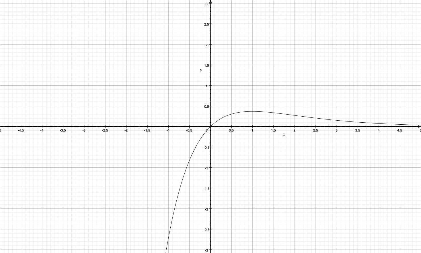
Easiest and very intuitive way to understand, that expression $te^{-\lambda t}$ goes to 0 as $t \to \infty$; is to look at its plot

so ,
\[\begin{align}
\mu &=\lambda \int\limits_{0}^{\infty}\frac{e^{-\lambda t}}{\lambda}dt
\\&=\int\limits_{0}^{\infty}{e^{-\lambda t}}dt
\\&=\frac{1}{\lambda}
\end{align}\]
Variance
\[\begin{align}
E[X^2]&=\int\limits_{0}^{\infty}t^2\lambda e^{-\lambda t}dt
\end{align}\]
now here
\[\begin{align}
u &= t^2
\\\& \ \ v&=-\frac{e^{-\lambda t}}{\lambda}
\end{align}\]
so,
\[\begin{align}
E[X^2]&=\int\limits_{0}^{\infty}t^2\lambda e^{-\lambda t}dt
\\&=\lambda\Big[-\frac{t^2e^{-\lambda t}}{\lambda}\Biggr|_{0}^{\infty} +\int\limits_{0}^{\infty}\frac{te^{-\lambda t}}{\lambda}dt\Big]
\end{align}\]
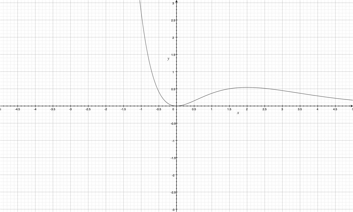
Graph for $t^2e^{-\lambda t}$ looks like this

Clearly the first term in the expression above is going to be simply 0 again.
\[\begin{align}
E[X^2]&=\int\limits_{0}^{\infty}t^2\lambda e^{-\lambda t}dt
\\&=\lambda\Big[-\frac{t^2e^{-\lambda t}}{\lambda}\Biggr|_{0}^{\infty} +2\int\limits_{0}^{\infty}\frac{te^{-\lambda t}}{\lambda}dt\Big]
\\&=2\int\limits_{0}^{\infty}{te^{-\lambda t}}dt
\\&=\frac{2}{\lambda^2}
\end{align}\]
using this for variance
\[Var(X)=\frac{2}{\lambda^2}-\frac{1}{\lambda^2}=\frac{1}{\lambda^2}\]
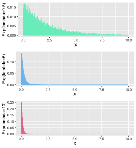
What does it look like

An example
Chef takes 5 minutes to make a burger . Whats the probability that chef will take 3 to 4 minutes to cook the next burger . You have all the tools at your disposal . Do it yourself .
What Next?
- Geometric, Negative Binomial , Hypergeometric
- Beta, Gamma, Weibull, Double Exponential
- Normal, Cauchy, Chi-Squared, t, F
Part 2 coming soon!
– Lalit Sachan [https://www.linkedin.com/in/lalitsachan/]
10 Dec 2019

Why I am writing this: I have seen this too many times now; while discussing gradient boosting machines that; some ML practitioners; don’t really understand what happens under the hood. Very often their understanding of boosting machines, starts with AdaBoost; and then kinda stops there.
Who is this best suited for : If you know what boosting machines are; but lack clarity on what happens under the hood.
Few things that I have not discussed [so, if you are here for a complete discussion; necessarily including what I have skipped, probably you should save your time and refer to some other source]:
- Relationship between $\eta$ and number of steps [boosted models ]
- In theory, individual models can be anything , but in most implementations you’d find these to be decision trees
- Individual models need to be weak learners
- I have not discussed line search here to find optimal fraction to multiply the predictions from $f_{t+1}$ before adding it to update $F_t$
Few mathematical ideas (Anchor Points) that, i will not be elaborating in this post are given; as is, below :
- Anchor Point 1: Gradient descent for parametric model requires us to change parameter by this amount in order to reach to the optimal value of cost function; starting at some random value of parameters :
- $\Delta\beta \rightarrow -\eta\frac{\delta C}{\delta\beta}$ , where $C$ is the cost function
- Anchor Point 2: Regression Problems
- Prediction model : $\hat{y}_i = F(X_i)$
- cost function : $\sum(y_i - F(X_i))^2$
- Anchor Point 3: Classification Problems
- Prediction model : $p_i =\frac{1}{1+e^{-F(X_i)}}$
- Other forms of the relationship written above
- $\frac{p_i}{1-p_i} = e^{F(X_i)}$
- $log(\frac{p_i}{1-p_i})=F(X_i)$
- Cost function : $-\sum[ y_i log(p_i)+(1-y_i)log(1-p_i) ]$
- Note : This cost is used for binary classification and is known as -ve log likelihood or binary cross entropy . For multi-class classification a more generic extension of the same; known as categorical cross-entropy, is used.
We’ll refer to these ideas in the post below wherever necessary.
We can start our discussion now about boosting machines . We’ll avoid having diagrams as much as we can. [In my opinion, that is another source of this huge misunderstanding. God bless those +,- diagrams of AdaBoost]
Bagging Methods
Bagging methods ( such as random forest ) make use of multiple individual models in a way that each individual model is independent of others . For example Prediction with bagging method is simply average of predictions coming from n individual predictors
\[F(X_i) =\sum\limits_{j=1}^{n}f_j(X_i)/n\]
In case of classification instead of $\hat{y_i}$ , this will be predicted probability $p_i$ where $f_j(X_i)$ will be hard class predictions [1/0].
In case of Random Forest, these individual predictors are decision trees .
Boosting Methods
In case of boosting machines there are two things which are different :
-
First : $F(X_i)= f_1(X_i)+f_2(X_i) ….. f_n(X_i)$
-
Second : These individual models are not independent of each other. In fact each subsequent $f_j(X_i)$ tries to improve upon the individual models added thus far. In other words; every subsequent model tries to ‘boost’ the performance of the model built before it.
How is $F(X_i)$ built ?
We just said that each $f_j(X_i)$ is added sequentially and it ‘boosts’ the model built before it. What exactly does this mean ?
Let’s consider that someone [somehow] has built $F(X_i)$ so far with t individual boosted models. We’ll represent the overall model also as $F_t(X_i)$ , to track its development .
\[F_t(X_i) = f_1(X_i)+f_2(X_i) ....... f_t(X_i)\]
How do we add, next boosted model $f_{t+1}(X_i)$ here to obtain $F_{t+1}(X_i)$ ?
$F_{t+1}(X_i) = F_t(X_i)+f_{t+1}(X_i)$
following ideas will helps us in understanding what this $f_{t+1}(X_i)$ is going to be
Gradient Boosting Machines and Cost in functional space
Cost for any kind of predictive problem is function of real values and predictions [or model outcomes]
\[C = \mathcal{L}(y_i,F_t(X_i))\]
Value of $\mathcal{L}$ for regression and classification is given at the beginning of this post above under anchor points 2 and 3.
Idea in Anchor Point 1, pertains to parameters. In context of gradient boosting machines; Key Idea is that instead of parameter change we are introducing small changes in our model $F_t$ , and this change is the new individual model being added in the sequence, that is $f_{t+1}$ . Following the idea of gradient descent :
\[f_{t+1} \rightarrow -\eta \frac{\delta C}{\delta F_t}\]
To be clear , $f_{t+1}$ is a model [ and is being used as a parallel to $\Delta\beta$ ]. It doesn’t make sense to say that it ‘equals’ the quantity on the RHS above.
It simply means that $f_{t+1}$ will be built as RHS as the target and it will change for each step $t$.
GBM for regression
For regression , considering sum of squared errors as cost function [ this can be any other exotic cost function too, thats another strength of GBMs; that they can work with custom cost functions as well]
\[C = (y_i -F_t)^{2}\]
We are not writing Xi explicitly anymore to keep things simpler
\(\begin{align}
f_{t+1} &\rightarrow -\eta \frac{\delta C}{\delta F_t}
\\ &\rightarrow -\eta [-2 *(y_i-F_t)]
\\ &\rightarrow \eta (y_i -F_t)
\end{align}\)
If you realise, $(y_i - F_t)$ is nothing but error of the model so far . An example with target table should make things clear .
| target for $f_1$ = $y_i$ |
Predictions of $f_1$ |
target for $f_2$ = $\eta(y_i - f_1)$ |
Predictions of $f_2$ |
Target for $f_3$ = $\eta(y_i -f_1-f_2)$ |
| $y_1$ |
$a_1$ |
$\eta(y_1-a_1)$ |
$b_1$ |
$\\eta(y_1-a_1-b_1)$ |
| $y_2$ |
$a_2$ |
$\eta(y_2-a_2)$ |
$b_2$ |
$\eta(y_2-a_2-b_2)$ |
| $y_3$ |
$a_3$ |
$\eta(y_3-a_3)$ |
$b_3$ |
$\eta(y_3-a_3-b_3)$ |
As you can see here , each subsequent individual model is building predictions for the errors which could not be handled by the models so far .
GBM for classification
It’s pretty intuitive and hence clear for regression that subsequent models that we are adding to build $F$ ; are regression models themselves.
Unfortunate and wrong extrapolation of the same idea that people end up taking, is that, in GBM for classification; individual models will be classificiation models. Which actually is not the case. [and is at the root of why I am writing this ]
Lets start with cost for binary classification in terms of $F_t$ [We’ll be using expressions from Anchor Point 3 to progress things here]
\(\begin{align}
C &= -\Big[ y_i log(p_i)+(1-y_i)log(1-p_i) \Big]
\\ &= -\Big[ y_i [log(p_i)-log(1-p_i)] + log(1-p_i) \Big]
\\ &= -\Big[ y_ilog(\frac{p_i}{1-p_i}) + log(1-p_i)\Big]
\\ &= -\Big[y_i*F_t + log\Big(1-\frac{1}{1+e^{-F_t}}\Big)\Big]
\\ &= -\Big[y_i*F_t + log\Big(\frac{e^{-F_t}}{1+e^{-F_t}}\Big)\Big]
\\ &= -\Big[y_i*F_t + log\Big(\frac{1}{1+e^{F_t}}\Big)\Big]
\\ &= -\Big[y_i*F_t - log(1+e^{F_t})\Big]
\end{align}\)
gradient expressions will be as follows :
\[\begin{align}
f_{t+1} &\rightarrow -\eta \frac{\delta C}{\delta F_t}
\\ &\rightarrow -\eta \Big[-\Big( y_i - \frac{e^{F_t}}{1+e^F_t}\Big) \Big]
\\ &\rightarrow -\eta \Big[-\Big( y_i - \frac{1}{1+e^{-F_t}}\Big) \Big]
\\ &\rightarrow -\eta \Big[-\Big( y_i - p_i\Big) \Big]
\\ &\rightarrow \eta (y_i-p_i)
\end{align}\]
Couple of key important details to understand from here
-
$\eta(y_i-p_i)$ , clearly is not a target for a classification model. Each individual model in GBM for classification is a regression model
-
Probability outcome from $F_t$ is NOT simply summation of probability outcomes from $f_1,f_2 ….$ . In fact the relationship is pretty complex as you can see here
- $p_t = \frac{1}{1+e^{-F_t}}$
- $F_{t+1} = F_t + f_{t+1}$
- $p_{t+1} = \frac{1}{1+e^{-F_{t+1}}} = \frac{p_t}{p_t+(1-p_t)e^{-f_{t+1}}}$
I hope this discussion brings some clarity into; how GBMs actually work [ especially for classification ].
09 Jul 2019

For a good time I believed that you can’t really give a long talk on feature engineering which will be relevant across multiple problem spaces. This belief originated from having seen people; calling problem specific special treatment of data; feature engineering . However , over the years I have unconsciously gathered pretty standard ways of treating different kind of features which are applicable irrespective of the kind of problem that you are working with. This of course doesn’t mean that there is no problem specific feature engineering , it simply implies that; you CAN have a good length discussion on generic feature engineering which applies well across different problems .
Sequence of different tips and tricks mentioned here doesn’t hold much meaning . I am simply writing/coding away things as and when I recall them here .
1. How to represent cyclic features
An intuitive example of such data columns are months or weekday numbers. Problem with simply giving them numbers is that the representation doesn’t really make sense . Why ?
Lets have a look :
| Month |
Coded_Value |
| January |
1 |
| February |
2 |
| March |
3 |
| April |
4 |
| May |
5 |
| June |
6 |
| July |
7 |
| August |
8 |
| September |
9 |
| October |
10 |
| November |
11 |
| December |
12 |
December isn’t really (12-1=11) months away from January. The next guy is January, they are just 1 month apart. Their numerical coding which we intend to use as a simple numeric column , doesn’t represent the same information.
A simple trick , in such cases of cyclical data is to use cyclical functions for encoding the values.
\[\text{months_sin} = sin(\frac{2*\pi*Months}{12})\]
In general this will be :
\[\text{x_sin} = sin(\frac{2*\pi*x}{max(x)})\]
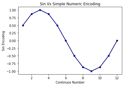
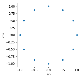
There is still a slight issue, simple plot of transformed values will clarify .

You can see that, now values start to turn up cyclically to have difference among them reducing as months near to end of year. The issue that I was talking about this approach , will become apparent if you look at values of month 2 and 4 . They have same values . The way to counter this is to use two cyclical functions ; both sin and cos. Any cyclic numeric column will be encoded as two columns, sin and cos transformations like this :
\[\text{x_sin} = sin(\frac{2*\pi*x}{max(x)}) \\
\text{x_cos} = cos(\frac{2*\pi*x}{max(x)})\]
They look truly cyclic now. All the values in 2 dimensions are different and retain distances among them as per their cyclic nature. :

Here is a quick function for the same :
def code_cyclic_features(data,columns,drop_cols=True):
  for col in columns:
    max_val=max(data[col])

    data[col+'_sin']=np.sin(2*np.pi*data[col]/max_val)
    data[col+'_cos']=np.cos(2*np.pi*data[col]/max_val)

    if drop_cols:
      del data[col]
  return data
2. Coding Categorical Features as dummies/flags
Ignoring the discussion where you can convert the categorical feature to some numeric representation without changing the sense of information .
Everybody starts coding categorical columns by creating n-1 dummies for n categories . However we should keep in mind that if any category doesn’t have enough observations/data, we won’t be able to extract consistent/reliable patterns from it. It’s a common practice to ignore such categories. You have to decide a frequency cutoff. There isn’t much point in searching the depths of internet to find a good value for this cutoff. Keep the tradeoff in mind , higher cutoff will lead to information loss and lower cutoff will lead to data explosion and overfitting.
Here is a quick python function which will enable you to create dummies with frequency cutoff.
def code_categorical_to_dummies(data,columns,frequency_cutoff=100):

    for col in columns:
        freq_table=data[col].value_counts(dropna=False)
        cats=freq_table.index[freq_table>frequency_cutoff][:-1]
        for cat in cats:
            data[col+'_'+cat]=(data[col]==cat).astype(int)

        del data[col]


    return data
3. Categorical Embeddings
Even when you use frequency cutoff , sometimes creating dummies results in data explosion as all of the categories might have good number of observation. Consider a data which has 11 columns where 10 are numeric and 11th column has 50 eligible categories . You’ll end up with 60 columns in the data. This could be a problem if you further decide to build a randomforest or gbm family models. You’ll decide the max_features parameter to be some random subset of these 60 columns in your data. By sheer number, the flag variables coming from a single column will be selected a lot more and , 10 numeric columns don’t get enough exposure due to inbuilt nature of the algorithm. We’d like to represent these flag variables at much lower dimensions than creating 50 separate columns in this scenario.
What comes to your rescue is embedding derived from neural networks which work as auto encoders . Here is an example in code which will help you in understanding the concept .
file = r'/Users/lalitsachan/Dropbox/0.0 Data/loans data.csv'
data=pd.read_csv(file)
data['State'].nunique()
Column State here has 47 unique values . We can create dummies but that will lead to having 47 one hot encoded columns . Lets see how we can come up with model driven embeddings for this column and bring down the dimension for the same .
dummy_data=pd.get_dummies(data['State'],prefix='State')
dummy_data.shape[1]
We’ll take the columns as our response as well. The network that we’ll be building [ an autoencoder] will be solving a pseudo problem. Its job is to take this one hot encoded representation [ dummy_data] and spit out the same values as the outcome. I call it a pseudo problem to solve because i am not really interested in the model which takes the input and spits it out as outcome perfectly. What is actually of interest to me is the compression that the input goes through in the intermediate layers of this model. Goal to build this pseudo network well is to ensure that this compression is not leading to information loss, that can only be said, if outcome of the network matches with the input.
from keras.models import Model,Sequential
from keras.layers import Dense,Input

embedding_dim=3
inputs=Input(shape=(dummy_data.shape[1],))
dense1=Dense(20,activation='relu')(inputs)
embedded_output=Dense(embedding_dim)(dense1)
outputs=Dense(dummy_data.shape[1],activation='softmax')(embedded_output)
model=Model(inputs=inputs,outputs=outputs)

embedder=Model(inputs=inputs,outputs=embedded_output)
We are going to use output of embedder as our transformed data. Embedding is being driven by predicting the response .
model.compile(optimizer='adam',loss='categorical_crossentropy',metrics=['accuracy'])
model.fit(dummy_data,y,epochs=150,batch_size=100)
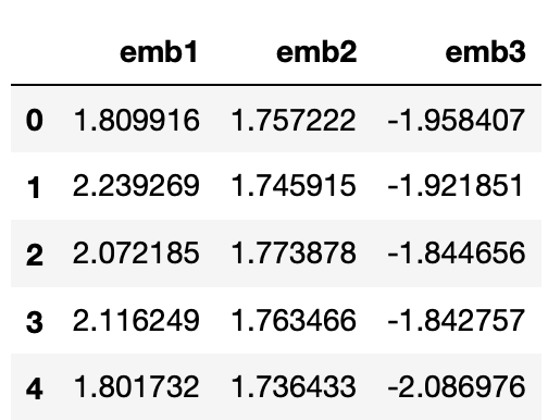
Once this is done , we can use embedder to get out transformed data, new low dimensional representation of 47 one hot encoded columns
low_dim=pd.DataFrame(embedder.predict(dummy_data),columns=['emb1','emb2','emb3'])
low_dim.head()

We can use the same trained embedder for test/val data as well.
4. Feature Selection using feature importance
Important Update :While this idea is good and sound. Implementation of feature importance in R/Python is not proper . And you should be cautious about using the same . You'll find more details here :
https://explained.ai/rf-importance/
It’s a common feature of many tree based ensemble method (both bagging and boosting), feature importance , which can be used for quick feature selection . But many sources failed to mention, where to draw the line. What level of feature importance should be set as cutoff , below which you can drop all the columns from further considerations .
Truth is , people don’t mention this because as such there is no fixed cutoff. And meaning of numeric value of feature importance can be data dependent. However a neat little trick can be used every time. You can add a random noise column as one of the features . Any column which gets its feature importance value below that, can be considered doing worse than white noise , which we know is not related to data and hence can be dropped.
Here is a quick example using one of the pre loaded datasets in sk-learn.
from sklearn.datasets import load_boston
boston=load_boston()

X=pd.DataFrame(boston.data,columns=boston.feature_names)
y=boston.target
We’ll add random noise to the data
X['white_noise']=np.random.random(size=(X.shape[0]))
Now lets build a quick random Forest model and check feature importance to see which features we can safely drop before further more detailed experiments with the data
from sklearn.ensemble import RandomForestRegressor
rf=RandomForestRegressor(n_estimators=200)
rf.fit(X,y)
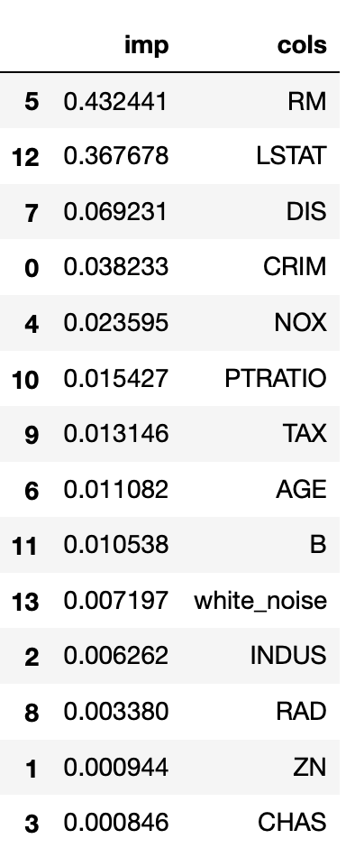
imp_data=pd.DataFrame({'imp':rf.feature_importances_,'cols':X.columns})
imp_data.sort_values('imp',ascending=False)

We can safely say that , we can drop columns INDUS, RAD, ZN, CHAS in context of predicting the target for this problem .
5. Ratio Features
As we move towards complex algorithms , need for manual feature creation goes down as many of the transformations can be learned by the algorithms of sufficient complexity ( Neural Networks , Boosting Machines ). Example of such transformations can be features created as interaction variables , log transformations or polynomials of original features in the data.
However ratio features are the ones which different algorithms are consistently bad at emulating . If you think that in context of the business problem that you are trying to solve; ratio of features in data can play definitive role then you should create them manually; instead of relying on any algorithm to extract that pattern.
A simple example of ratio variable can be utilisation of credit cards [ratio between expense and limit]
You can find a detailed discussion about what kind of feature transformation different algorithms can emulate and what they can not : here
Few notes on the takeaways/followups .
- This is not an exhaustive list by any means. I discussed few things which I see; are not commonly discussed or are generally looked over. I’ll make additions if I recall something else.
- Whenever I discussed one of the tricks, I skimmed over other details. For example , when we were talking about categorical embeddings , we can very well first ignore categories which have low frequencies , create dummies for the rest and then go for categorical embeddings .
- Feel free to let me know if you’d like me to add some discussion as part/addition to the list above.
